Shaping our bones
 Figure 1: A Kayan woman with neck rings. Image Steve Evans.
We know that applying a force to a bone during its development can influence its growth and shape. In ancient China parents bound girls' feet to prevent growth, as small "lotus sized" feet were considered beautiful. In a few African and Asian cultures an elongated neck is considered a sign of beauty. Women of the Kayan people (Burma, Myanmar) begin to wear neck coils from as young as two and continue to add successive brass coils as they grow (see figure 1). The effect of this technique is an elongated neck, but vertebrae do not actually elongate. The weight of the coils instead applies enough pressure on the shoulder blades to eventually deform them, generating the illusion of a long neck.
But can we use our understanding of how developing bone reacts to mechanical forces to help people suffering from diseases that lead to bone deformities? Researchers have investigated this question for years. They have developed mathematical models to help predict the shape of our bones. Using these models it is now possible to predict, for example, how the femur of a child will grow over the next few months by analysing the child's walking patterns. The mathematical models of bone growth will eventually make it possible to prevent bone deformities in children with diseases such as cerebral palsy and hip dysplasia.
How do bones grow?
Long bones grow longer by gradually turning cartilage into bone. This is exactly what happens at the extremities of the long bones, where cartilage templates, called growth plates, are slowly replaced by bone. Figure 2(i) illustrates the growth plates in the femur — these layers of cartilage, at both ends of the shaft, are responsible for most of the growth in length of our long bones.
 Figure 2: (i) The femoral growth plates are shown in blue at both ends of the bone. (ii) The zoom on the right shows the areas of the ossification process in a longitudinal section of the developing femur.
Figure 2(ii) shows a longitudinal section of the developing femur, as we see it through a microscope. It shows how cartilage cells slowly turn into bone. First, cartilage cells rest in the cartilage matter. They then start to rapidly reproduce (a) and then they enlarge, mainly in the longitudinal direction (b). The calcium constituting our bones starts to deposit in the ossification area, so that the cells are surrounded by mineralised matter (c) and finally turn into bone (d). Note that the process by which bone grows in girth, called appositional growth, is different.
Bone formation is regulated by biological factors, such as genes, hormones and nutrients, and by mechanical factors, including muscle forces and forces due to the contact of bones at the joints. Biological and mechanical factors are closely linked together. However, for the purpose of this article we will keep them separated. This simplification allows us to describe the growth rate of a bone, $\dot{\epsilon}$ (which describes the change in length of the bone relative to the initial length of the bone over time), as the sum of a biological component, $\dot{\epsilon}_b,$ and a mechanical component, $\dot{\epsilon}_m$: $$\dot{\epsilon}=\dot{\epsilon}_b+\dot{\epsilon}_m. \;\;\;\;\;\;\;\;\;\;\;\;\;\;\;\;\;\; \mbox{(1)}$$ The biological growth rate $\dot{\epsilon}_b$ represents the growth that occurs due to intrinsic genetic and hormonal regulation, while the mechanical growth rate $\dot{\epsilon}_m$ represents the growth due to the loads on bone, that is muscle and joint forces. Assuming that the biological growth rate is constant, we can concentrate only on the effects of the mechanical loads on bone growth.
How do mechanical loads affect bone growth?
During normal development, most loads acting on the bones are cyclic and multiaxial, that is, they act in multiple directions. Forces applied on the bone during walking are a clear example of this. They are cyclic because each step we take is similar to the one before, and they are multiaxial as muscles and joints are pulling and pushing the bone in different directions.
As a reaction to external forces applied on the bone, internal forces are produced between the particles of the bone itself. A measure of these internal forces is called stress. Quantitatively, stress measures the intensity of a force per unit area. For the simple case, for example a body pushed or pulled by two forces acting in opposite directions at its extremities, the stress within the body can be obtained by dividing the total force by the cross-sectional area of the body.
 Figure 3: There are three normal stresses acting in the direction of the axes and six shear stresses acting in the planes perpendicular to the axes.
But forces acting on bones are usually multiaxial and this makes a full description of the stress more complicated. Embedding our bone in a coordinate system (with x, y and z axes), we would normally need to define nine parameters: three normal stresses (acting in the direction of the axes of our coordinate system) and six shear stresses (acting in the planes perpendicular to the axes of our coordinate system). See figure 3. However, there are many different ways in which we can embed the bone in a coordinate system and fortunately there is always one in which the shear stresses turn out to be zero. The stress state is now described in terms of only three normal stresses. These stresses are called principal stresses.
Using the principal stresses we can now define two stress components. The first, called hydrostatic stress, is responsible for a change in an object's volume without changing its shape. A balloon provides an example: if you inflate or deflate it, then the volume of the balloon will change, but its shape will stay the same. The second stress component, called octahedral shear stress, is responsible for changes in an object's shape without changes in its volume: if you close the balloon's opening, then you can change its shape by squishing it, but this won't change its volume.
Figure 4 shows a representation of the two stress components in their pure form. Pure hydrostatic compressive stress (shown on the left) is a result of equal pressure applied along the three principal directions. This stress is represented by $\sigma=\sigma_1=\sigma_2=\sigma_3.$ By convention, the $\sigma_i$ are negative numbers (a positive $\sigma$ would correspond to hydrostatic tensile stress, which pulls rather than pushes the body). Hydrostatic stress is measured by a single number made up of the three principal stresses: $$\sigma_H=(\sigma_1+\sigma_2+\sigma_3)/3.$$ Octahedral shear stress represents the distortion of a body when it is pressed in one direction and as a result is pulled outward in the other two directions. The numerical value measuring octahedral shear stress is given by the formula: $$\sigma_S=(\sqrt {(\sigma_1-\sigma_2)^2+(\sigma_2-\sigma_3)^2+(\sigma_3-\sigma_1)^2})/3.$$
 Figure 4: A representation of pure hydrostatic compressive stress and pure octahedral shear stress. σ1, σ2 and σ3 represent the principal stresses. The original configuration of our balloon is shown in blue. Pure hydrostatic compressive stress (on the left) represents equal pressure applied to a balloon in the three principal directions. Pure octahedral shear stress (on the right) represents the distortion of the balloon when pressed in one direction (the balloon will be pulled outward in the other two directions).
Hydrostatic stress and octahedral shear stress are called stress invariants, because they are defined in terms of the principal directions and therefore independent of the coordinate systems you choose. This property makes them particularly useful in describing stresses resulting from multiaxial loading conditions. We can use these two stresses to define the stress state at the growth plate during bone development.
In 1987 the mechanical engineer Dennis R. Carter, Professor at Stanford School of Engineering, and his colleagues studied the influence of cyclic and multiaxial loads on bone growth and ossification. They proposed that cyclic hydrostatic compressive stress inhibits bone growth and ossification, while cyclic octahedral shear stress promotes them. According to this theory, the mechanical component $\dot{\epsilon}_m$ in the formula above can be expressed as a combination of the lowest compressive hydrostatic stress ($\sigma_H$) and the highest octahedral shear stress ($\sigma_S$) that occur due to the different forces that are applied to the bone in a cycle of action (for example, during a single step, we apply several different forces on the bone in order to achieve the motion, which is a cyclic action). $$\dot{\epsilon}_m=Max\{\sigma_S\}+0.5 Min\{\sigma_H\}. \;\;\;\;\;\;\;\;\;\;\;\;\;\;\;\;\;\; \mbox{(2)}$$ The octahedral shear stress is always positive and promotes growth and ossification. The hydrostatic compressive stress is always negative and it inhibits growth and ossification. This equation gives a mathematical model of long bone growth, known as the mechanobiology theory of bone growth. (The term "mechanobiology" refers to the regulation of biological processes by mechanical factors.)
How do we model bone growth?
The mechanobiological theory can be used to simulate growth using a computer model of the bone. First, we represent the bone of interest as consisting of many small pieces, called elements. For each element we record the material and structural properties of the corresponding piece of bone. These will define how the bone reacts to certain forces. The computer model will calculate the stress state within the bone and the resulting deformation of the bone for each single element and use this information to simulate overall growth of the bone. The more elements there are, the more accurate our modelling is. This type of computer model is known as a finite element model.
Our computer simulation of bone growth is based on six steps.
Step 1: First we create a geometric representation of our bone. In the example shown in figure 5.1 we've created a 3D representation of a femur (to keep things simple, we concentrate only on one end of the femoral bone). Bone is represented in green and blue (representing cortical and trabecular bone respectively, a more dense and a less dense bone we have in our body), growth plate is represented in purple. The transition zone, which simulates the actual material transition from cartilage to bone described above, is represented in orange.
Step 2: In the second step we simulate loads coming from the muscles and joints being applied to our virtual bone. In the example in Figure 5.2, different hip joint contact forces generated during walking, represented by red arrows, press on the head of the femur. Mathematically, these forces are represented by vectors.
Step 3: In step three we calculate the resulting stresses in each of the elements representing the growth plate. Then, using equation 2, we calculate the mechanical contribution to the bone growth, $\dot{\epsilon}_m$, at the growth plate due to the forces applied on the bone. Finally, we calculate the bone growth rate using equation 1. The value of the biological component $\dot{\epsilon}_b$ is taken to be twice the mechanical component $\dot{\epsilon}_m$. This estimate comes from experimental observations, which shows that bone grows between 50\% and 80\% of its normal size when there is no mechanical loading.
Figure 5.3 shows the resulting pattern of the mechanical growth rate $\dot{\epsilon}_m$ at the femoral growth plate region (view from above): in red are the areas with increased growth rate and in blue the areas with reduced growth rate.
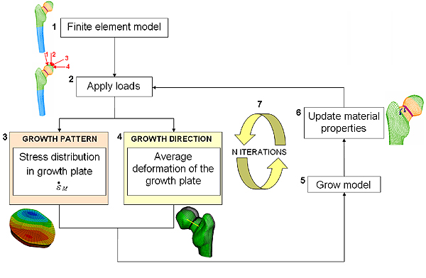 Figure 5: A flow chart of the computer model.
Step 4: The fourth step is to calculate the direction of bone growth. Researchers previously observed that when a load is applied, bone grows in the direction in which the cartilage of the growth plate has deformed. We approximate the deformation of the femoral growth plate by the average deformation of the neck of the femur, and consider this as the growth direction of our femur.
Step 5: In step 5 we simulate bone growth by enlarging the elements of the growth plate according to the growth rate and in the direction of growth calculated in steps 3 and 4 respectively.
Step 6: In step 6 we simulate gradual bone formation by turning a layer of the growth plate into the transition zone and a layer of the transition zone into bone. Our bone model now has a slightly different material composition and shape. By applying steps 2 through to 6 again, we can simulate long bone growth over time (figure 5.7), according to the stress distributions on the growth plate and its deformations. We can do this until the entire growth plate region has turned into bone.What does our model predict?
Mathematical models such as this one can be used not only for femurs, but also for any other long bone and with any cyclic or intermittent loads. They predict how the skeletons of humans and animals change during their lives. These applications can help us understand, for example, the architectural changes of human bones from childhood to adulthood, or how the human locomotor apparatus (bone structure and muscle activity) differs from that of other two-footed primates, for example bonobos and chimpazees. The models can also help explain the evolution of human and animal species.
But the models are also useful tools in predicting bone deformities due to diseases. For example, the particular model presented above has allowed us to define how bone deformities progress in children with cerebral palsy. We observed four children who each walked with different gait patterns. For each child we estimated hip joint contact loads and muscle forces acting on the femur during walking. We then calculated the stresses in the growth plate and implemented the mechanobiological theory over time, to predict how the femur would grow over the next five months. The model predicted that children with cerebral palsy would develop bone deformities at the proximal femur and that these deformities would be more extreme for the children with the most abnormal gait patterns. This suggests that the altered gait patterns in children with cerebral palsy can cause bone deformities.
Mechanobiological models can be used to predict bone growth for other diseases too, including osteoarthritis, scoliosis, hip dysplasia and others. Once we understand how bone deformities develop, we may be able to correct the deformity before it affects function and develop treatment regimes to maintain the normal mechanical environment of the growing bone.
About the author

Alessandra Carriero is a Post-doctoral Research Associate in the Department of Bioengineering at Imperial College London. She is currently recipient of a Global Research Award from the Royal Academy of Engineering and working in the Material Science Division at the Lawrence Berkeley National Laboratory (California, US). She received her MSc from Politecnico di Milano (2005) in Biomedical Engineering and a PhD from Imperial College London (2009) in Bone Biomechanics. She has previously been a Research Assistant at Trinity College Dublin and a Post-doctoral Research Fellow at ETH Zürich. Her research uses computational methods, animal experiments and clinical collaborations to determine the influence of mechanical loads on bone during growth and in disease.
Comments
Raven
Can you change your lower jawbone after applying pressure to it?
Joe Dell
I just wonder what about the microstructure?