
In Making the grade: Part I we considered what the gradient of a curve might mean, and how to find it by appealing directly to the definition. In particular, we used direct arguments - which were really quite involved - to calculate the gradients of the curves x2 and sin(x). To perform this kind of calculation every time we need to calculate such a gradient would be a nightmare - especially if we had a complicated function. In this article we think about the process of manipulating the algebraic expressions with which we usually describe functions in order to perform this calculation. This is differentiation as we know and love it!

The other kind of gradient.
Image DHD Photo Gallery
The whole point of having a set of formal rules is to allow us to temporarily forget the exact meaning and to concentrate on calculation. After all, we can only concentrate on a few things at a time. Of course, it is vital to keep the meaning in the back of our minds, as a check that the answer is sensible. Furthermore, by having a set of rules disjoint from a particular context, we can apply the rules in many different settings.
The rules allow us to differentiate just about any algebraic expression we care to write down. Of course we have to decide which formal rules to apply in a given situation, and in what order. Sometimes it is not clear which rule we should apply - there are a number of things we could do correctly. What then to do? How should we decide? As we shall see, the answer to these questions is surprising and illustrates the intimate way in which calculus and algebra interact.
Calculating gradients using the calculus
In the previous article we calculated the gradient by considering the change in divided by the change in
  , that is,
 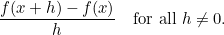 |
(1) |
 we obtained
 ![\[ \frac{f(x+h)-f(x)}{h} = \frac{(x+h)^2-x^2}{h} = \frac{x^2+2xh+h^2-x^2}{h} =2x+h. \]](/MI/e89d418a4fc0cc1d9c02ee6b194d2eb2/images/img-0005.png) |
 tends to zero, either positive or negative, gave
  as the derived function, or derivative, of
  .
.
Let’s generalize this and consider  where
where  is any natural number, that is,
  . Of course, we have already considered the cases when
  (the straight line) and when
  (the quadratic).
In order to calculate (1) when we need to consider
![\[ \frac{f(x+h)-f(x)}{h} = \frac{(x+h)^ n-x^ n}{h}. \]](/MI/8119585b03e30cbaf7b87c19be034d33/images/img-0006.png) |
To simplify this we need to expand out the term
![\[ (x+h)^ n. \]](/MI/8119585b03e30cbaf7b87c19be034d33/images/img-0007.png) |
When we do this for small values of we get
![\[ \begin{array}{lcc} (x+h)^0 & = & 1, \\ (x+h)^1 & = & x+h, \\ (x+h)^2 & = & x^2 + 2xh + h^2, \\ (x+h)^3 & = & x^3 + 3x^2h + 3xh^2 + h^3, \\ (x+h)^4 & = & x^4 + 4x^3h + 6x^2h^2+ 4xh^3 + h^4, \\ (x+h)^5 & = & x^5 + 5x^4h + 10x^3h^2 + 10x^2h^3+ 5xh^4 + h^5. \\ \end{array} \]](/MI/8119585b03e30cbaf7b87c19be034d33/images/img-0008.png) |
We could do this by hand for other values of by multiplying out the brackets, but this is tricky, time-consuming and it is all too easy to slip up. In fact, there is a very regular pattern to the coefficients of the terms in the expansions above. If we ignore the  ’s and
  ’s we obtain the pattern known as Pascal’s Triangle, part of which is shown below.
![\[ \begin{array}{c} 1 \\ 1\ 1 \\ 1 \ 2 \ 1 \\
1 \ 3 \ {\color{blue} 3} \ {\color{blue} 1} \\ 1 \ {\color{red} 4} \ {\color{red}6 } \ {\color{blue} 4} \ 1 \\ 1 \ 5 \ {\color{red} 10} \ 10 \ 5 \ 1 \\ \end{array} \]](https://plus.maths.org/content/sites/plus.maths.org/files/issue27/features/sangwin/mtgp2equation.png)
 is generated by adding the
  and
and  above it. Similarly, the red
  is obtained by adding the and
  above it.
In general, the number in the position  in from the left on the
  th row is given by the formula
![\[ ^{n}C_ k = \frac{n!}{(n-k)!k!}. \]](/MI/f53196368b3ffb9fc7c768f66b453632/images/img-0003.png) |
These numbers are known as the binomial coefficients, because  is the coefficient of
  when we expand
  . This result is known as the binomial theorem and it allows us to exploit this pattern to write as
![\[ (x+h)^ n = x^ n + ^{n}C_1x^{n-1}h + ^{n}C_2x^{n-2}h^2 + ^{n}C_3x^{n-3}h^3\\ + ... + ^{n}C_{n-2}x^2 h^{n-2} + ^{n}C_{n-1}x h^{n-1} + h^ n. \]](/MI/f53196368b3ffb9fc7c768f66b453632/images/img-0007.png) |
We are currently interested in calculating the quantity (1) when  . To do this we note that, for all values of ,
![\[ ^{n}C_1=\frac{n!}{(n-1)!} = \frac{ n \times (n-1) \times (n-2) \times ... \times 2 \times 1}{(n-1) \times (n-2) \times ... \times 2 \times 1} = n. \]](/MI/f53196368b3ffb9fc7c768f66b453632/images/img-0009.png) |
Using this we have
![\[ \frac{(x+h)^ n -x^ n}{h} = \frac{(x^ n + ^{n}C_1 x^{n-1}h + ^{n}C_2 x^{n-2}h^2 + ... + h^ n) - x^ n }{h}\\ \\ = nx^{n-1} + h \times (\mbox{stuff}). \]](/MI/f53196368b3ffb9fc7c768f66b453632/images/img-0010.png) |
We don’t really need to know exactly what the " stuff" is in the above expression in this case. This is because it is multiplied by  , and letting tend to zero wipes out all these terms. What we are left with is the function
  So we express this result as
 |
(2) |
whenever is a natural number (ie,  ). If
). If  in this argument we have
![\[ \frac{d}{dx} x = 1, \]](/MI/f53196368b3ffb9fc7c768f66b453632/images/img-0016.png) |
which confirms that the gradient of the straight line  is constant.
This result may be expanded so that (2) holds whenever  is a real number, although this takes a little more work.
To take another example, let  (remember that
  for all
  ). So we have the formula
![\[ f(x)=x^0=1. \]](/MI/419868ef6a5add2f646b580cf090985c/images/img-0004.png) |
![\[ \frac{d}{dx} x^0 = 0.x^{-1} = 0. \]](/MI/419868ef6a5add2f646b580cf090985c/images/img-0005.png) |
Constructing functions
Functions are fundamental to modern mathematics and you simply can’t avoid using them. The idea of a function is to take two sets of objects known as the inputs and outputs. To every input the function assigns a unique output:
![\[ \mbox{input} \quad \rightarrow \quad \fbox{Function} \quad \rightarrow \quad \mbox{output.} \]](/MI/0273f5ce9dae319d146682bb6e63b299/images/img-0001.png) |
Most often the inputs and outputs are sets of numbers, such as the real line. The function is also most often described using a formula, in the form of an algebraic expression. This is exactly the idea of a function we have considered so far, although we haven’t been explicit about it! This is also the way we will continue to think about functions.
The reason we pause now to think of functions in a more abstract way is simply to acknowledge that a function is much more general than a formula. In fact, the function  introduced in the previous article was built from two formulae bolted together. Recall these were
![\[ |x|:= \left\{ \begin{array}{ll} x, & x\geq 0\\ -x, & x < 0. \end{array} \right. \]](/MI/0273f5ce9dae319d146682bb6e63b299/images/img-0003.png) |
The trigonometric functions  ,
,  , etc. are constructed with reference to a geometrical shape - in this case a circle of radius
  . Other ways of building functions involve an infinite series (that is a sum) or a sequence of formulae. We won’t consider these in this article, but just concentrate on how we can build up functions from simple operations.
Let us assume our input is a number  . The simplest operations we could perform on our variable are the arithmetic ones. That is addition, multiplication and the two inverse operations of subtraction and division. Because we can manipulate the formulae using algebra we can often write one formula in different ways.
For example, consider
 |
(3) |
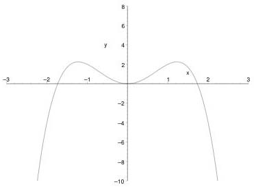
Figure 1: The function (3)
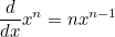
We can think of  as
as  multiplied by
  . Both these functions are shown in Figure 2. Try to imagine what happens when you multiply the values on each graph together.
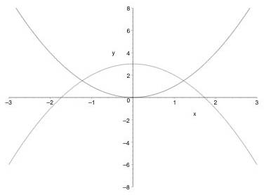
Figure 2: The functions x2 and 3-x2
Alternatively, to calculate  we might subtract
  from
from  . The graphs of these functions are shown in Figure 3. Since
 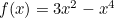 we can recreate Figure 1 by subtracting one from the other. No doubt there are other ways of constructing the same function
  .
.
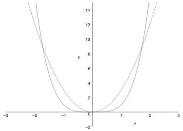
Figure 3: The functions x4 and 3x2
Functions can also be applied in order, one after the other, as in
![\[ \mbox{input} \quad \rightarrow \quad \fbox{Function 1} \quad \rightarrow \quad \fbox{Function 2} \quad \rightarrow \quad \mbox{output.} \]](/MI/ff861499f319e93653c5bcaf928a974e/images/img-0001.png) |
![\[ g(u)=u(3-u) \]](/MI/ff861499f319e93653c5bcaf928a974e/images/img-0002.png) |
![\[ u(x)=x^2. \]](/MI/ff861499f319e93653c5bcaf928a974e/images/img-0003.png) |
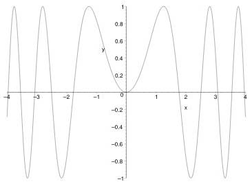
Figure 4: The function sin(x2)
Of course, we have to ensure that any output from Function 1 is a legitimate input for Function 2. In this case we say the two functions have been composed. For example, a function such as sin(x2) can be thought of as the function that maps x to sin(x) applied to the result of the function that maps x to x2. Note that the
order really does matter here and sin(x2) and sin(x)2 are very different functions: see Figures 4 and 5.
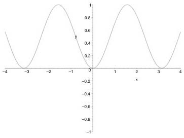
Figure 5: The function sin(x)2
Given the numerous ways we could express a function such as (3), how should we go about differentiating it? This is the question we address in the rest of this article.
Linearity of the differential calculus

You don't always get the same result if you do things in a different order!
The first general rule allows us to calculate the derivative of two functions which have been added together. If we want to find the gradient of f(x)+g(x) we simply find the gradients of f(x) and g(x) separately and then add the results. In a more condensed (and easier to read) form this may be expressed as:
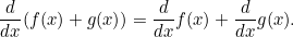 |
(4) |
 is multiplied by a constant
  then
then 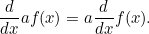 |
(5) |
 by breaking it down into constant multiples of
  for various
  , and then applying (2). This is powerful indeed.
Example
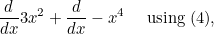
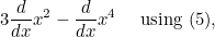
For example, to calculate the gradient of the function  defined in (3), we write this as the unfactored form
  and can then apply the rules as follows:
 |
 |
 |
|||
 |
|
 |
|||
|
|
 |
Any book on calculus will contain many similar examples and exercises for you to practice.
Before we go any further, we need a word of warning about notation. In particular, there are many ways of writing the derivative of a function at the point  . Different authors have different preferences. So far we have used the notation
![\[ \frac{d}{dx} f(x), \]](/MI/8f60641e26caa0df720627c16fea640e/images/img-0010.png) |
which was promoted by Leibnitz. Another notation, used by Newton, has two forms:
![\[ f’(x) \mbox{ or }\dot{f}(x). \]](/MI/8f60641e26caa0df720627c16fea640e/images/img-0011.png) |
Although neater in some circumstances, it is very easy to misread a dot or apostrophe and so care is needed. We will use both kinds of notation.
General rules
Linearity, which is expressed in the formulae (4) and (5), together with our result (2) allows us to calculate the derivative of any polynomial by breaking it into separate parts. In fact (4) and (5) involve two general functions. What would be really useful would be two rules which allow us to calculate gradients when general functions are multiplied or composed together, that is to say, rules which allow us to find
 |
(6) |
and
 |
(7) |
where  and
and  are any differentiable functions. We make a huge assumption in believing that such general rules really exist. However, if they do then the rules applied to
  in various different ways must respect the result (2). For example,
  may be written as
  , or as
  . The rule for (6), if it exists, must give
  when applied to each of these ways of writing . Otherwise we could obtain different answers for the derivative. So, we look at different ways of writing as a product, and try to find a rule which is consistent, at least for these.
Let’s start by defining  and split this up into
![\[ f(x) = x^ m \quad \mbox{and}\quad g(x)=x^{n-m}, \]](/MI/a592c0616c5a1ccaaa465280c21b06a6/images/img-0011.png) |
so that
![\[ F(x)=f(x)\times g(x). \]](/MI/a592c0616c5a1ccaaa465280c21b06a6/images/img-0012.png) |
We know using (2) that
![\[ F’(x) = nx^{n-1}, \quad f’(x)=mx^{m-1}, \quad \mbox{and}\quad g’(x)=(n-m)x^{n-m-1}. \]](/MI/a592c0616c5a1ccaaa465280c21b06a6/images/img-0013.png) |
Our task is to write  in terms of
  and
and  as an attempt to gain some insight into what the general rule (6) might be. That is, we write
where A and B are unknown functions of x. Now, using algebra we can confirm that
Thus if we take  and
and  we have a correct general rule whenever we split
  into (8). This rule may be written as
 |
(8) |
Immediately, by linearity, it follows that (8) holds for any polynomial.
Can we find a rule for general functions, like  , which are not polynomials? Certainly, if a general rule exists, when we apply this to
  , the rule should reduce to (8). In fact, the rule for general functions turns out to be precisely (8), and is better known as the Product Rule.
Similarly, if we write
![\[ F(x)=x^{nm}=(x^{n})^ m \]](/MI/b67fb850272e45127a30b6a3ae95e8ec/images/img-0007.png) |
and
![\[ f(x)=x^ n, \quad \mbox{and}\quad g(x)=x^ m, \]](/MI/b67fb850272e45127a30b6a3ae95e8ec/images/img-0008.png) |
we have  . Again, we know using (2) that
![\[ F’(x) = nmx^{nm-1}, \quad f’(x)=nx^{n-1}, \quad \mbox{and}\quad g’(x)=mx^{m-1}. \]](/MI/b67fb850272e45127a30b6a3ae95e8ec/images/img-0010.png) |
Our task is to write  in terms of
  and
and  as an attempt to gain some insight into what the general rule (7) might be. But
which suggests a general rule
 |
(9) |
There's a rule for everything - even chains!
Image DHD Photo Gallery
In fact, the rule for general functions turns out to be precisely (9) again, and is better known as the Chain Rule.
These rules are really very comprehensive, and proofs may be found in any text book on advanced calculus. A huge range of functions can be build up, and conversely decomposed, using these rules. When trying to differentiate a complicated function, the method is to decompose it into simpler components, and work with these separately. The derivatives of these simple parts can be recombined using the general rules to find the derivative of the original function. For completeness we state these rules again below, in two common forms of notation and for each give a worked example.
The chain rule
The following rule allows us to differentiate functions built up by compositions. Let’s assume that we have some function which we can choose to write as a composition  . Let
. Let  , then
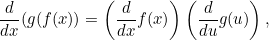 |
(10) |
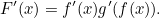
or, using alternative notation,
![\[ (g(f(x)))’ = f’(x)g’(f(x)). \]](/MI/1254f7535d97c793e6517ba5bde7d97d/images/img-0004.png) |
Example:
Let us return and consider the function  . Writing
  and
and  , we already know that
![\[ \frac{d}{du} \sin (u)=\cos (u)\quad \mbox{and}\quad \frac{d}{dx} x^2=2x. \]](/MI/1254f7535d97c793e6517ba5bde7d97d/images/img-0008.png) |
Substituting these into (10) gives
![\[ \frac{d}{dx} \sin (x^2) = 2x \cos (x^2). \]](/MI/1254f7535d97c793e6517ba5bde7d97d/images/img-0009.png) |
Note: we have  here, not
  , as we have .
The product rule
Functions can be built up by components which are multiplied together. For example,  . To differentiate this we use the formula
 |
(11) |
or, using alternative notation,
![\[ (f(x)\times g(x))’ = f’(x)g(x) + f(x)g’(x). \]](/MI/3d9b560a1bafa35374fde3d03554fabd/images/img-0003.png) |
Example:
This time consider the function  . This can be decomposed into the two functions
  , each of which we know how to differentiate. Therefore we can use the rule (11) immediately to write
![\[ \frac{d}{dx} x^2\sin (x) = 2x\sin (x) + x^2\cos (x). \]](/MI/3d9b560a1bafa35374fde3d03554fabd/images/img-0006.png) |
The quotient rule
Functions can be built up by components which are divided one by the other. Actually, since dividing by  is identical to multiplying by
  to work out the derivative of
  we could just apply the product rule to
  , and the chain rule to
  composed with
  . But it is convenient to have a separate rule for this, which is
![\begin{equation} \frac{d}{dx} \left[\frac{f(x)}{g(x)}\right] = \frac{g(x)[\frac{d}{dx} f(x)] - \left[\frac{d}{dx} g(x)\right]f(x)}{g(x)^2}, \end{equation}](/MI/55b33cee3f8be3c3385ab5e284209731/images/img-0007.png) |
(12) |
or, using alternative notation,
![\[ \left[\frac{f(x)}{g(x)}\right]’ = \frac{g(x)f'(x)-g'(x)f(x)}{g(x)^2}. \]](/MI/55b33cee3f8be3c3385ab5e284209731/images/img-0008.png) |
Example:
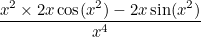
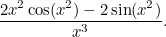
This time we differentiate  . We know how to differentiate
  , even though it is itself a composition. We applied (10) to this and it has derivative
  . Using (12) gives
![$\displaystyle \frac{d}{dx} \left[\frac{\sin (x^2)}{x^2}\right] $](/MI/55b33cee3f8be3c3385ab5e284209731/images/img-0012.png) |
 |
![$\displaystyle \frac{x^2 [\frac{d}{dx} \sin (x^2)] - [\frac{d}{dx} x^2]\sin (x^2)}{(x^2)^2} $](/MI/55b33cee3f8be3c3385ab5e284209731/images/img-0014.png) |
|||
 |
|
 |
|||
|
|
 |
Applying the rules
To finish, instead of giving lots of different examples (which can be found in any calculus text), we take the reverse approach and think about one example in more detail. In particular, we return to the function  . We know from the previous result (2) that the derivative of is
  . We write this as
![\[ \frac{d}{dx} x^4 = 4x^3. \]](/MI/5df544dec8fb11436087255288f3f00b/images/img-0003.png) |
Using the rules of algebra we could write this function in a number of ways. We can also think of  . Alternatively,
  or even
  .
.
Taking the first of these, since the derivative of  is
is  , we may apply the product rule to give
![\[ \frac{d}{dx} (x^4) = \frac{d}{dx}(x^2\times x^2) = 2x \times x^2 + x^2 \times 2x = 2x^3 + 2x^3 = 4x^3. \]](/MI/5df544dec8fb11436087255288f3f00b/images/img-0009.png) |
We could also apply the product rule to one of the other representations of this function. In particular, we could calculate the derivative as
![\[ \frac{d}{dx} (x^4) = \frac{d}{dx}(x\times x^3) = 1 \times x^3 + x \times 3x^2 = x^3 + 3x^3 = 4x^3. \]](/MI/5df544dec8fb11436087255288f3f00b/images/img-0010.png) |
Similarly we could think of being a composition of two functions: as " -squared, all squared", that is to say,
  . In this case we may apply the chain rule to see that
![\[ \frac{d}{dx} (x^4) = \frac{d}{dx}((x^2)^2) = 2(x^2) \times 2x = 4x^3. \]](/MI/5df544dec8fb11436087255288f3f00b/images/img-0013.png) |
Notice that in each case we get the same correct answer.
We need not stop there. For example, we could write  and apply the quotient rule. If we do this we have
![\[ \frac{d}{dx} \left(\frac{x^6}{x^2}\right) = \frac{x^2\times \frac{d}{dx} (x^6) - \frac{d}{dx} (x^2) \times x^6}{(x^2)^2} = \frac{x^2\times 6x^5 - 2x\times x^6}{x^4} = \frac{6x^7-2x^7}{x^4} = 4x^3. \]](/MI/5df544dec8fb11436087255288f3f00b/images/img-0015.png) |
The point is that in order to find the derivative of we may do anything algebraically legitimate and apply any of the rules for differentiation correctly. The way we choose to find the derivative, as long of course as it is applied correctly, does not matter. We could ask: How many ways are there of differentiating ? Can you think of others?
About the author

Chris in the Volcanoes National Park, Hawaii, Summer 2003
Chris Sangwin is a member of staff in the School of Mathematics and Statistics at the University of Birmingham. He is a Research Fellow in the Learning and Teaching Support Network centre for Mathematics, Statistics, and Operational Research. His interests lie in mathematical Control Theory.
Chris would like to thank Mr Martin Brown, of Thomas Telford School, for his helpful advice and encouragement during the writing of this article.