Maths in a minute: Linear regression

A linear regression tries to estimate a linear relationship that best fits a given set of data. For example, we might want to find out how the number of tropical storms has changed over the years. In this case, we can plot the number of storms against time. The linear regression will find the straight line that best fits the plotted data, and calculate several statistics indicating how well the line fits the data and whether the slope of the line is significantly different from zero (i.e., whether there is a real trend or not). (See this article for more on the tropical storm example.)

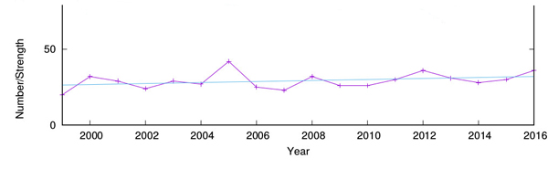
Yearly tropical storms. The blue line indicates the result of a linear regression on the number of storms over time.

In general, when you perform a linear regression, a dependent variable (say $y$ , the number of tropical storms in our example) is assumed to be linearly dependent on one or more explanatory variables (say $x_1$ , $x_2$ , etc, up to $x_ n$ ). The general equation for the linear relationship is

$y = a_0+a_1x_1+a_2x_2+ ...+ a_ nx_ n.$

Given a set of observed values for the dependent variable $y$ and corresponding explanatory variables $x_1$ to $x_ n$ , the linear regression then estimates values for the model parameters $a_0$ to $a_ n$ such that the total error (i.e., the differences between the observed values $y$ and the model predicted values $\hat{y} = a_0+a_1x_1+a_2x_2+ ... +a_ nx_ n$ ) is minimised.

For example, in the case of tropical storms the dependent variable is the number of storms each year (hurricanes), and the (single) explanatory variable is time (year). For a set of 18 observations from the Monthly Storm Reports, one for each year from 1999 to 2016, a linear regression results in the following estimated model:

$hurricanes = -637.9+0.3323 \times year.$

In this data set, the observed number of hurricanes for the year 2001 is 29. However, the model predicted value for this year is $-637.9+0.3323\times 2001 = 27.03$ . In other words, the error is $29-27.03 = 1.97$ . In the model estimation, the values of the parameters were chosen in such a way that the total error (summed over all years) is minimised (in reality, a linear regression actually minimises the sum of squared errors).

Linear regression can help you spot trends in your data.

A statistic that is often used to indicate how well the estimated model fits the given data is the coefficient of determination, denoted $R^2$ , which measures the proportion of the variance in the dependent variable that is actually explained by the explanatory variable(s). This value is usually on a scale from zero to one, with zero indicating no explanatory value (i.e., complete unpredictability) and one indicating full explanatory value (i.e., complete predictability). The $R^2$ value in the regression performed here is $R^2=0.11$ , which is low. This indicates that the estimated models have very little explanatory power, and that the data is mostly random rather than having a linear dependence on time.

Finally, a linear regression analysis also tests the null hypothesis that the slope of the regression line is zero (i.e., that there is actually no dependence of the dependent variable on the explanatory variables). The statistic calculated to decide whether to accept or reject this null hypothesis is the p-value. This statistic (a value between zero and one) indicates the probability that the data is the way it is under the assumption that there is no dependence. Another way to put this is to say that the p-value indicates the probability of making a mistake when rejecting the null hypothesis (i.e., the probability of rejecting a true hypothesis).

A standard threshold (or significance level) used for the p-value is 0.01, or a 1% probability of rejecting a true hypothesis. This means that any p-value that is larger than 0.01 is not considered enough statistical evidence to reject the null hypothesis. Sometimes a more "forgiving" significance level of 0.05 (or 5%) is used, but the main idea is that the higher the p-value of the regression, the more likely it is that the slope of the linear model is not significantly different from zero. (You can find out more about p-values and significance levels in this article.)

Do it yourself

If you'd like to perform your own linear regression, you might want to use the R program. For example, for the hurricane data (after extracting the number of storms for each year from the public database), the regression can be performed with the following R commands:

year<-c(1999,2000,2001,2002,2003,2004,2005,2006,2007,2008,2009,2010,2011,2012,2013,2014,2015,2016)
hurricanes<-c(20,32,29,24,29,27,42,25,23,32,26,26,30,36,31,28,30,36)
myModel<-lm(hurricanes ~ year)
summary(myModel)
predict(myModel)

The summary command prints out a summary of the linear regression, including the estimated values for the model parameters, the $R^2$ value and the p-value, and several other statistics. The predict command provides the model predicted values (with which the blue line in the figure above was plotted).

About the author

Wim Hordijk is a computer scientist currently on a fellowship at the Konrad Lorenz Institute in Klosterneuburg, Austria. He has worked on many research and computing projects all over the world, mostly focusing on questions related to evolution and the origin of life. More information about his research can be found on his website.