Stokes's phenomenon: An asymptotic adventure

Life is the art of approximation. If we took into account all the details of every aspect of the things we experience, we'd never get anywhere. We need to be careful about which things to ignore, though, because if those details contain a proverbial devil, they can come back to bite us.

Mathematicians have learnt this lesson many times. A great example is Stokes' phenomenon, a problem which originated nearly 200 years ago with a question about rainbows, and has generated an entire field of mathematics. Indeed, this year the Isaac Newton Institute in Cambridge ran a virtual research programme on the topic, bringing together some of the best minds in the field. The problem concerns very small — exponentially small — quantities, which over time and space can grow to be exponentially large. Understanding these potentially explosive quantities is essential in all sorts of areas beyond maths: from building jet engines to theoretical physics.

Below the rainbow

The problem started in 1838 with the then Astronomer Royal George Biddell Airy, who was interested in rainbows. If you are lucky, when you look closely at a rainbow you will see one or more faint arcs below the main bow that are predominantly green, pink and purple. Airy was interested in these supernumerary fringes not so much for their own sake, but because a similar fringing effect occurs in optical lenses which, as an astronomer using telescopes, Airy wanted to understand.

A rainbow with supernumerary fringes. Photo: Johannes Bahrdt, CC BY-SA 4.0.

The Airy function

The Airy function $Ai(r)$ is a solution to the differential equation

$\frac{d^2y}{dx^2}-xy=0.$

It is given by the integral

$y=Ai(x)=\int _0^{\infty } \cos {\frac{\pi }{2}\left(\frac{t^3}{3}+xt\right)}dt.$

The intensity of the light as you you cut perpendicularly across the rainbow is related to the square of the Airy function. Find out more here.

In the early 17th century René Descartes had explained how the main rainbow comes about using a theory which imagines light as consisting of rays. "But the ray theory of light doesn't predict that [supernumerary fringes] exist, so you can't model what they are," says Chris Howls of the University of Southampton and co-organiser of the Newton Institute programme. "Airy used a wave theory of light and this naturally gives rise to supernumerary fringes."

Airy wrote down a mathematical formula, now called the Airy function, from which you can read off the intensity of the light of the main bow and its supernumerary arcs, and also the location of the arcs, as you cut across the rainbow with a line that's perpendicular to it. "Airy wanted to compute where these supernumerary fringes were because that would help improve the optics of telescopes," says Howls.

The problem with Airy's function was that it was difficult to evaluate. Given a particular value of $x$ it was hard to work out $Ai(x).$ At first, Airy painstakingly evaluated the function for values of $x$ between $-4$ and $4$ at intervals of $0.2,$ using something called the method of quadratures. Eleven years later he improved his results using a method that had been suggested to him by the mathematician Augustus de Morgan: he approximated the function using infinitely long sums.

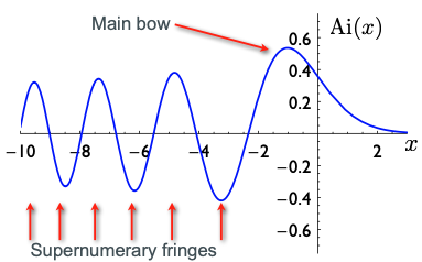
With today's methods it's possible to evaluate the Airy function and plot it. The main bump on the right corresponds to the main rainbow and the smaller bumps going off to the left to the supernumerary fringes. (The square of the Airy function gives the intensity of the light). This figure is from a talk by Chris Howls and Adri Olde Daalhuis that was given given at the Isaac Newton Institute.

The power of powers

The idea that an infinitely long sum can be useful at all may seem strange at first, so let’s look at an example. Think of the exponential function

$f(x)=e^ x,$

where $e$ is Euler’s number $e=2.718281....$

The function comes with what is called a Taylor series given by the infinite sum

$S(x)=1 + x + \frac{x^2}{2 \times 1} + \frac{x^3}{3 \times 2 \times 1} + \frac{x^4}{4 \times 3 \times 2 \times 1} + \frac{x^5}{5 \times 4 \times 3 \times 2 \times 1 } + ...,$

which involves powers of the variable $x$ .

Now given any particular value of the variable $x$ , you can never add up all the terms in this series (you don’t have an infinite amount of time) but you can add up the first, say, $n$ terms, giving you what is called a partial sum. It turns out that the result you get is an approximation of $e^ x$ : the larger $n$ (i.e. the more terms you include in your partial sum) the better the approximation. Indeed, you can get as close an approximation as you like by making $n$ sufficiently large (i.e. including enough terms in the partial sum). Mathematicians say that the series $S(x)$ converges to the value of $f(x)$ for all $x$ .

Now to estimate the value of $e^ x$ at, say, $x=2$ we simply substitute $x=2$ in the first few terms of the Taylor series (also called a Maclaurin series). Using the first 5 terms, we get

$1+2+\frac{4}{2\times 1}+\frac{8}{3\times 2\times 1}+\frac{16}{4\times 3 \times 2 \times 1}=7.$

The actual value of our function $f(x)$ at $x=2$ is $f(2)=e^2\approx 7.4.$

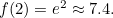
So in this case, even just using 5 terms of the Taylor series gives a reasonable approximation of the value of the function at $x=2$ .

Taylor series exist for a whole class of functions. And Taylor's theorem even tells you how far the approximations you get from them are from the actual value of the function.

Taylor failure

This is great in principle, and using the Taylor series of his function (you can see it in Airy's paper) Airy was indeed able to evaluate the Airy function for values of $x$ in a range from $-5.6$ to $5.6.$ But there was still a hitch. Although the Taylor series of the Airy function converges to the function itself, it does so very slowly. "It turns out that you need to calculate thirteen or fourteen terms in that series representation before you even get the first [supernumerary] fringe," says Howls. "In 1838 that was incredibly difficult to do because you had to do the calculations by hand and that just wasn't practical."

Airy function plot and cubic approximation

The blue curve is the Airy function and the red curve the approximation you get from three terms of its Taylor series. You can see the approximation only captures the first bump on the right, corresponding to the main rainbow. This figure is from a talk by Chris Howls and Adri Olde Daalhuis that was given given at the Isaac Newton Institute.

To find an easier way of approximating the Airy function, the mathematician George Gabriel Stokes in 1850 decided to play with fire. He enlisted the help of series that don't converge.

Satanic series

As you can easily imagine, not all series converge to a finite value. A simple example is the series

$1+2+3+4+5....$

As you include more and more terms in your partial sums, the results you get become larger and larger, eventually exceeding all bounds — they don’t approach a finite value. Such a series is said to diverge to infinity.

Divergent series are treacherous beasts you can play all sorts of tricks with — see this article for some examples. In 1828, not so long before Stokes started his work on Airy's function, the Norwegian mathematician Niels Henrik Abel had described divergent series as an "invention of the devil" and declared it shameful to "base on them any demonstration whatsoever."

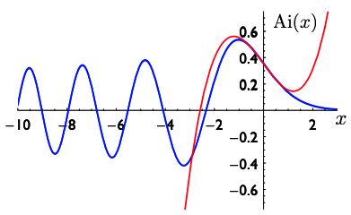
But Stokes, in his quest to approximate Airy's function, was not deterred. A deep look at the mathematics of Airy's function led him to consider divergent series that nevertheless delivered a good approximation to the function (the series is a little bit complicated to write down, but you can see it here). The trick here is knowing where to stop. As the series Stokes considered diverges to infinity, if you look at too long a partial sum, its value will be huge and miss the corresponding (finite) value of Airy's by miles. However, if you consider a partial sum that's just short enough, the approximation will be close.

When you add up more and more of the initial terms of a sum that diverges to infinity, you get larger and larger results, eventually exceeding all bounds. However, Stokes knew that for the divergent sums he was dealing with, taking exactly the right number of terms would give you a good approximation to Airy's function.

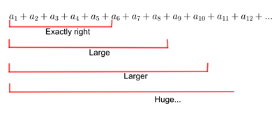
Stokes' ingenious approach gave him a way of approximating the values of Airy's function with "extreme facility" for relevant values of $x$ , so he had essentially nailed the practical problem of figuring out the supernumerary fringes of a rainbow. In the graph below the the blue curve represents the actual Airy function, while the red curve comes from Stokes' approximation. As you can see, red matches blue very closely. The only mismatch occurs around the point $x=0$ , on either side of which the red curve shoots off to infinity. As far as the rainbow is concerned, this discrepancy doesn't matter much, because what we're interested in is the behaviour of the Airy function along the bits representing the supernumerary fringes of the rainbow, to the left of $x=0$ .

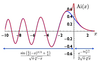
The blue curve is the actual Airy function and the red curve Stokes' asymptotic approximations. The formulae give the descriptions of each part of the approximation. This figure is from a talk by Chris Howls and Adri Olde Daalhuis that was given given at the Isaac Newton Institute.

The word asymptotic here refers to the fact that the approximation works only for large enough positive values of $x$ , and small enough negative ones. (This is akin to what happens with straight-line asymptotes you might have learnt about at school. See here for a formal definition of "asymptotic" and here for what's probably the most famous asymptotic result of all of mathematics, the prime number theorem.)

But despite this success, Stokes wasn't at all happy. The two parts of his approximation were described by two very different mathematical expressions (given in the plot above). This bothered Stokes. "What Stokes wanted to know was, how do you go from one [expression to the other]?", says Howls. "This question vexed him for a lot of his career, from 1850 to 1902." The answer Stokes eventually found showed that, when it comes to asymptotic approximations, tiny exponential terms can suddenly "be born" and then grow to attain dominance. Find out more in the second part of this article.

About this article

This article relates to the Applicable resurgent asymptotics research programme hosted by the Isaac Newton Institute for Mathematical Sciences (INI). You can see more articles relating to the programme here.

Marianne Freiberger is Editor of Plus. She interviewed Chris Howls in July 2021.

This article is part of our collaboration with the Isaac Newton Institute for Mathematical Sciences (INI), an international research centre and our neighbour here on the University of Cambridge's maths campus. INI attracts leading mathematical scientists from all over the world, and is open to all. Visit www.newton.ac.uk to find out more.