Intriguing integrals: Part I

You might also like to read the second part of this article.

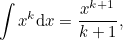
What is the integral of $x^ k$ ? If you're up to speed with your calculus, you'll know the answer off by heart. It's

$\begin{equation} \label{eq:int_ log}\int x^ k \mathrm{d}x = \frac{x^{k+1}}{k+1},\end{equation}$

(1)

for $k\neq -1$ , and

$\begin{equation} \label{eq:int_ log} \int x^{-1}\mathrm{d}x = \int \frac{1}{x}\mathrm{d}x = \ln (x).\end{equation}$

(2)

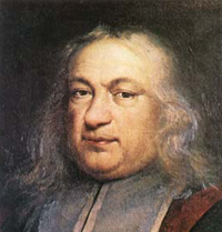
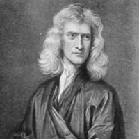
Pierre de Fermat, 1601-1665.

But can you prove that this is true? In this article we'll derive (1) from first principles, using an ingenious method devised by the mathematician Pierre de Fermat in the 17th century. In the second part of this article, we'll examine the surprising fact that, at a symbolic level, the answer to $\int x^ k\mathrm{d}x$ might better be written as

$\int x^ k\mathrm{d}x = \frac{x^{k+1}-1}{k+1}.$

The integral of x²

Let's start by deriving the integral

$\int x^ k\mathrm{d}x = \frac{x^{k+1}}{k+1}$

for $k=2$ by calculating the area under the graph of $f(x)=x^2$ without using calculus, that is from first principles.

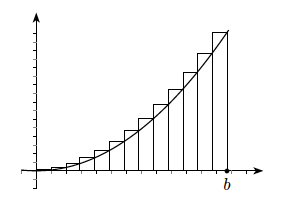
One approach is to use the above diagram, where we have approximated the area between the curve, the $x$ -axis and the vertical line at $x=b$ by a sequence of $n$ rectangles. The rectangles are constructed on intervals on the $x$ -axis of length $\frac{b}{n}$ . The height of each rectangle is the maximum value of the curve on the corresponding interval. In the case of $x^2$ this maximum value occurs at the right hand end of each interval. For the $i$ th interval this right hand end point is $x_ i=\frac{ib}{n},$ and the corresponding value of the function is $f(\frac{ib}{n})=\left(\frac{ib}{n}\right)^2.$ The area of the $i$ th rectangle is therefore

$A_ i= \frac{b}{n} \times \left(\frac{ib}{n}\right)^2=\frac{i^2b^3}{n^3}.$

The total area of the rectangles is

$\sum _{i=1}^ n A_ i = \sum _{i=1}^ n \frac{i^2b^3}{n^3} = \frac{b^3}{n^3} \sum _{i=1}^ n i^2.$

Using the sum

$\label{eq_ sun_ n_ squared} 1^2+2^2+3^2+\cdots +n^2=\sum _{i=1}^ n i^2 = \frac{1}{6}n(n+1)(2n+1)$

and simplifying, we can show that the total area of the rectangles equals

$b^3 \left(\frac{1}{3}+\frac{1}{2n}+\frac{1}{6n^2} \right).$

This overestimates the area under the curve, as each rectangle pokes out above the curve. But by a similar method we could estimate the area of $f(x)=x^2$ from below, using rectangles with height equal to the minimum value of the function on the corresponding interval. If we repeat this analysis we have the area as

$b^3 \left(\frac{1}{3}-\frac{1}{2n}+\frac{1}{6n^2} \right).$

Combining these two estimates for the area under the graph, we have

$b^3 \left(\frac{1}{3}-\frac{1}{2n}+\frac{1}{6n^2} \right)\leq A \leq b^3 \left(\frac{1}{3}+\frac{1}{2n}+\frac{1}{6n^2} \right).$

As $n\rightarrow \infty$ both of these estimates converge to

$\frac{b^3}{3} \leq A \leq \frac{b^3}{3}.$

Since these estimates trap the area between them, the only option is that

$A = \int _{0}^ b x^2 \mathrm{d}x = \frac{b^3}{3},$

which gives us the required expression

$\int x^ k\mathrm{d}x = \frac{x^{k+1}}{k+1}$

for the case $k=2$ .

The integrals of x^k for k>2

It is clear that this method could, in principle, be extended to find

$\int x^ k\mathrm{d}x$

for all positive numbers $k=1,2,3,\cdots$ . However, the method relies on being able to sum series of the form $\sum _{i=1}^ n i^ k$ . We know how to do this for $k=2$ , but doing it for $k>2$ is a different matter.

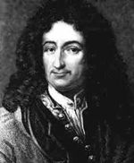
Isaac Newton, 1643-1727.

Before Isaac Newton's discovery of the fundamental theorem of calculus, which allows integrals to be evaluated in practice as anti-derivatives, resorting to such sums was the only way to calculate integrals as areas. Newton and Gottfried Wilhelm von Leibniz made very significant advances in the development of calculus as a systematic set of tools. This work began at least with Archimedes and has a continuous history (see reference [2] below). For example, work on the integration of rational functions was collected together by the mathematician G.H. Hardy in 1916 (see reference [3]), but it was only with the advent of computer algebra systems that an algorithm was developed which determined whether an elementary expression could be integrated symbolically at all (see reference [4]).

One of these incremental developments was discovered by Fermat who devised a method for calculating

$\int x^ k\mathrm{d}x$

where $k$ is any positive rational number. Here we will only consider the case when $k=1,2,\cdots$ . (See reference [1] below for more on this method)

First, choose a positive whole number $k$ and a positive real number $b>0$ . Fermat's method uses rectangles of unequal width. To start, fix an integer $n$ and a number $r$ with $0<r<1$ . Now consider rectangles whose vertical sides meet the $x$ -axis at points of the form $r^{i}b$ for $i=0\cdots n$ .

The graph of f(x)=x² with b=0.8, and with x_i=rⁱb. Use the sliders to change the value of r (and therefore the widths of the rectangles), and to change the value of n to see the position of the nth rectangle. Created with GeoGebra

Now, the $x$ -coordinate of the right hand end of the $i$ th rectangle is $r^ ib$ . The $x$ -coordinate of the left hand end of the $i$ th rectangle is $r^{i+1}b$ . If we subtract the $x$ -coordinates of the ends of rectangles to get the width, we have $r^ ib-r^{i+1}b=b(1-r)r^ i$ . The height of the $i$ th rectangle is $(r^ ib)^ k$ . The total area of these rectangles is then

$\sum _{i=0}^{n-1} b(1-r)r^ i\times (r^ ib)^ k = b^{k+1}(1-r)\sum _{i=0}^{n-1} (r^{k+1})^ i.$

The sum in the right hand side of this expression is a geometric progression, which we can evaluate using the standard formula

$\sum _{i=0}^{n-1} (r^{k+1})^ i=\frac{1-(r^{k+1})^ n}{1-r^{k+1}}.$

The total area is thus

$b^{k+1}(1-r)\frac{1-(r^{k+1})^ n}{1-r^{k+1}}.$

If we let $n\rightarrow \infty$ , we have an infinite number of rectangles which together fill the area between $0$ and $b$ . Using the sum of an infinite geometric progression, we get a total area of

$b^{k+1}(1-r)\frac{1}{1-r^{k+1}}.$

Gottfried Leibniz, 1646-1716.

Now notice that the more rectangles we use, the better our approximation of the area under the curve. Letting the widths of all the rectangles tend to zero, and therefore their number to infinity, will give us the area of the curve as a limit. The width of $i$ th rectangle is $b(1-r)r^ i$ , which tends to $0$ as $r\rightarrow 1$ . (Use the sliders in the figure above to see how the widths of the rectangles change as $r$ tends to 1, and how far to the left the rectangles extend as $n$ gets larger.) Therefore, the area under the curve is equal to

$\lim _{r \rightarrow 1} b^{k+1}(1-r)\frac{1}{1-r^{k+1}} = b^{k+1}\lim _{r \rightarrow 1}\frac{1-r}{1-r^{k+1}}$

It's not immediately obvious what this limit might be, but we can use a clever trick to find out. Using our geometric progression again, we know that

$1+r+r^2+r^3+\cdots +r^ k = \frac{1-r^{k+1}}{1-r}.$

This means that

$\frac{1-r}{1-r^{k+1}}=\frac{1}{1+r+r^2+r^3+\cdots +r^ k}.$

Substituting this into our limit above gives

$b^{k+1}\lim _{r \rightarrow 1}\frac{1-r}{1-r^{k+1}} = b^{k+1}\lim _{r \rightarrow 1} \frac{1}{1+r+r^2+r^3+\cdots +r^ k}= \frac{b^{k+1}}{1+1+1+\cdots +1} = \frac{b^{k+1}}{k+1},$

which gives us the integral $\int x^ k \mathrm{d}x$ as expected.

Have a go yourself

If this article has inspired you to do some calculus, here are a couple of problems for you:

Use the method described here and the result

$\sum _{k=1}^ n k^3 = \frac{1}{4}n^2(n+1)^2$

to find the area under $f(x)=x^3$ .
Use apply Fermat’s method of unequal rectangles to calculate the area under $f(x)=\frac{1}{x}$ between $x=1$ and $x=2$ .

You might also like to read the second part of this article.

References

[1] W.G. Bickley, §1324. An adventure with limits, The Mathematical Gazette, 22(251):404-405, October 1936.

[2] C.H. Edwards, The Historical Development of the Calculus, Springer-Verlag, 1979.

[3] G.H. Hardy, The integration of functions of a single variable, Tracts in Mathematics and Mathematical Physics. Cambridge University Press, 1916.

[4] R.H. Risch, The problem of integration in finite terms, Transactions of the American Mathematical Society, 139:167-189, May 1969.

Chris Sangwin is a member of staff in the School of Mathematics at the University of Birmingham. He has written the popular mathematics books Mathematics Galore!, with Chris Budd, and How round is your circle? with John Bryant, and edited Euler's Elements of Algebra.

Intriguing integrals: Part I

The integral of x2

The integrals of xk for k>2

Have a go yourself

References

The integral of x²

The integrals of x^k for k>2