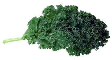
A kale leaf is crinkled up around its edge.

Picture a curved line. That's not so hard – I'm sure you're already imagining a smoothly curving line drawn on a blank white page, perhaps a circle, or a sine curve wiggling up and down across the page.

Now picture a curved surface. Again, not so hard. You might think first of a something simple like a cylinder or a sphere. Or perhaps something a bit more complicated, like a frilly kale leaf (a good illustration of a hyperbolic surface), a dimpled ball or a flag rippling in the wind.

In a previous article, Kissing the curve, we saw that understanding curvature of one-dimensional lines and two-dimensional surfaces is all a matter of osculating (kissing) circles of the curves in a flat plane. (For surfaces we consider the curves formed by intersecting the surface with planes perpendicular to the tangent planes.)

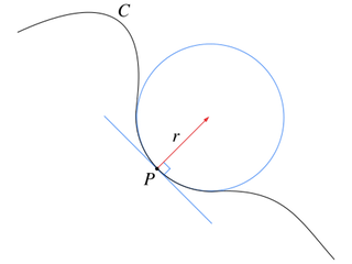
The osculating circle of this curve at the point P. The curvature at this point is 1/r where r is the radius of the osculating circle.

Mathematicians and physicists are interested in the curvature of higher-dimensional objects. And we are affected by such curvature every day: the gravity we feel is the result of the curvature of the four-dimensional spacetime of our Universe. But how do you describe curvature of something that has more than two dimensions?

Manifolds

It's easy for us to picture a one-dimensional curve drawn on a flat plane. And we can easily picture a two-dimensional surface in three-dimensional space. But for most of us picturing anything in higher dimensions is impossible. Where our brains and imagination fail, we can use maths to paint the picture for us.

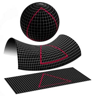
We need to generalise the idea of a surface or a line to higher dimensions. Most of the lines we come across, whether they are curved or straight, look locally like a straight line (this is the basis for calculus). A surface, whether curved like a ball, rippling like a flag or flat as a table-top, viewed close up looks like a flat plane. (CGI in movies uses this concept in order to approximate a complicated surface with lots of tiny flat pieces – you can read more in It's all in the detail.) Both lines and surfaces are examples of manifolds – mathematical objects that viewed up close look like ordinary flat space (where points are located using perpendicular coordinate axes), which is known as Euclidean space.

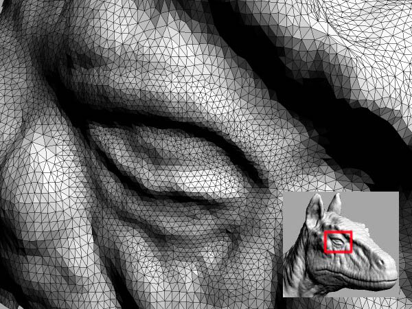
This image is actually made up of millions and millions of shaded triangles.

The tangents to a curve (which you can think of as a one-dimensional manifold) are straight lines. Surfaces (two-dimensional manifolds) also have tangent planes. In fact, the tangent space of an n-dimensional manifold at any point is a Euclidean space of dimension n, . And just as we understood curvature for lines and surfaces, the curvature of a manifold is the amount it differs from its flat tangent space.

In order to understand curvature in this way, the tangent space has to vary smoothly across the surface. If a line or surface has a sharp kink, there is no way to define curvature at this point as the tangent line (or planes) abruptly change from one side of this point to the other, and isn't defined at the kinky point. So in order to consider curvature of manifolds, we consider manifolds that too have smoothly varying tangent spaces across the manifolds. These are called Riemannian manifolds, after the mathematician Bernard Riemann who extended this notion of curvature to many dimensions. (Actually, the precise definition of a Riemannian manifold is that the inner product – the operation that defines distances and angles – for the tangent spaces varies smoothly across the manifold.

The sphere has positive curvature, the saddle has negative curvature and the flat plane has zero curvature. A circle drawn on the sphere would have a smaller area than one drawn on the flat plane. While a circle drawn on the saddle would have a greater area than one drawn on the flat plan. (Image courtesy NASA.)

Curvature

We saw in the last article that there is a notion of curvature, called Gaussian curvature, that is intrinsic: it can be detected by a 2D resident living on the surface; you don't need an outside perspective to see it. The resident would be able to detect the positive, negative or flat curvature of the surface by summing the interior angles of triangles: positive curvature corresponds to the interior angles adding to more than 180° (such as on the surface of the Earth), a negative curvature to the interior angles adding to less (a surface similar to that of a crinkly kale leaf) and flat (0) curvature to the angles adding exactly 180°.

Similarly, you can understand the curvature of higher-dimensional Riemannian manifolds intrinsically, without caring how the manifold is embedded in any larger space. The simplest measure of curvature on Riemannian manifolds is scalar curvature, , defined for each point in the manifold. This describes how a small ball in the manifold centred on , differs in volume from an equivalent ball in Euclidean space.

To understand this let's go back to something we can picture more easily – a ball of radius on a surface is made up of all the points that lie within a distance of , as measured within the surface, from the centre point : a filled circle. Since you have to measure the distances within the surface, it might not be the same distance you would measure between these two points in the Euclidean space that contains the surface. This is why the circle in the surface is not necessarily the same as the equivalent circle in Euclidean space (ie, a filled circle with centre and radius , where the distances are measured in Euclidean space).

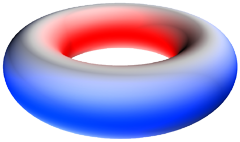
The torus has regions with different curvature: on the outside of the torus curvature is positive (blue), on the inside it's negative (red), and at the top and bottom circles it's zero (grey). (Image from Mark L. Irons.)

At a point with positive curvature the ball on the manifold will be smaller than the equivalent ball of radius in Euclidean space: a circle cut from a flat piece of paper will have to be folded or crumpled to cover the equivalent circle on the surface of a sphere. If the surface has negative curvature at a point , the volume of the ball will be larger than for Euclidean space: to create crocheted versions of hyperbolic surfaces , more and more stitches are needed as the radius increases. (You can read more in Chaotic crochet and Knitting by numbers.)

Our examples of a sphere and hyperbolic surfaces have constant scalar curvature over the whole surface. But you don't have to look far to find a surface with varying curvature: a torus has equal amounts of positive and negative curvature over the whole surface, as shown in the image on the right.

The scalar curvature assigns a single real number to each point – it defines a scalar field across the manifold. And the scalar curvature is enough to completely describe the curvature of a two dimensional manifold (ie. a surface). However in more than two dimensions we need something a little more complicated.

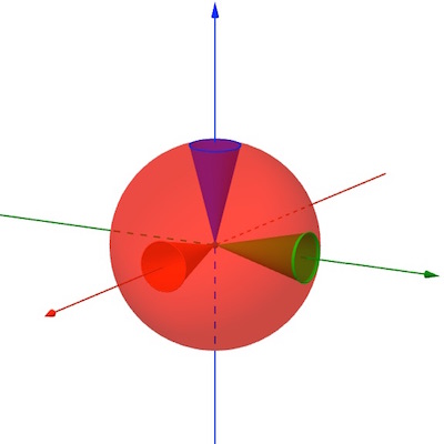
The Ricci curvature describes how conical regions in the manifold differ in volume from the equivalent conical regions in Euclidean space.

Instead of considering how the volume of a whole ball within the manifold differs from one in Euclidean space, we consider the volume of just a sliver of the ball – an angular sector or cone centred around some direction from the centre of the ball. The Ricci curvature, , describes how the sliver of a ball at point in direction in the manifold differs in volume from the equivalent angular sector in Euclidean space. For any point on the manifold, we can define the value of the Ricci curvature in any direction from that point: for any direction we can look at the difference between the volumes of a sliver in the manifold, and a sliver in Euclidean space, in that direction. Unlike the simpler scalar curvature which defines a scalar field across the manifold, the Ricci curvature is a tensor field, that is it is defined for all directions from each point on the manifold. (You can read more about tensors in Feeling tense about tensors?)

The Ricci curvature comes into play when you are considering manifolds of three or more dimensions. For a two-dimensional manifold the Ricci curvature gives you the same information as the scalar curvature – the Ricci tensor has the same value in all directions for any point: . But in three or more dimensional manifolds it is possible for a point to have positive Ricci curvature in one direction and negative Ricci curvature in another.

Moving on up

In four and higher dimensions we need a more complex description of curvature. We're now in territory we can't visualise anymore and we need maths to describe these objects and properties. But we can get a sense of one description of curvature in these higher dimensions by viewing it as an extension of the definition of Gaussian curvature we used to understand the curvature of surfaces.

Consider a plane in the tangent space of the higher-dimensional manifold at some point . Then for any direction in the tangent plane from , there is a unique geodesic curve within the manifold emanating from in the direction. (A geodesic curve is a generalisation of straight lines on a flat plane or great circles on the globe of the world – a unique curve that give the shortest distance between two points in a manifold.) Then, even if our manifold has four or more dimensions, we can sweep out a two-dimensional surface within the manifold, made up of all the geodesic curves within the manifold emanating from as we move through all the directions in the tangent plane.

We can calculate the Gaussian curvature for this surface for any tangent plane at a point . This is called the sectional curvature for the tangent plane . Giving the sectional curvatures for all planes tangent to the manifold at a point describes the curvature of a manifold at completely. The sectional curvatures for all tangent planes at every point in a manifold describe a tensor field.

Equivalently, you can completely describe the curvature of a manifold using the Riemannian curvature tensor. Rather than focussing on the Gaussian curvature of surfaces defined by tangent planes, Riemannian curvature describes how curvature twists tangent vectors as they move around a manifold. (A vector represents a magnitude – its length – and direction.)

Think of a triangle drawn on a flat piece of paper. Imagine attaching a small vector to one of the corners (lying on the paper – as it's a tangent vector to this surface) and move it around the triangle, preserving the angle it makes with each side as it goes (this is called parallel transporting a vector along each line). The vector will have the same orientation when it returns to its starting point, it will be pointing in the same direction.

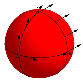
The angle of the tangent vector attached to the sphere changes direction as it is parallel transported along lines of latitude and longitude.

Now consider a sphere, and to make it easier to keep track of things consider it with the same lines of latitude and longitude we use as coordinates on Earth. Start at the point on the equator of longitude and latitude (point A on the image on the right) and consider a tangent vector to the surface at that point, pointing directly north. Then travel directly north, along the line of longitude, dragging the tangent vector with you, keeping it at the same angle to the line of longitude. At the North Pole (point N in the image) your tangent vector is now pointing in the direction of the line of longitude at , perpendicular to the line of longitude east.

Now travel down the line of longitude east, dragging the tangent vector and keeping it perpendicular to the direction of travel. When you arrive back at the equator, at the point longitude, latitude of east (point B), the tangent vector will now be pointing east along the equator.

Travel back along the equator to your starting spot at latitude, longitude (point A), dragging the tangent vector with you and keeping it parallel withthe equator. When you return to your starting point your tangent vector is now pointing due east. The vector has twisted through an angle of 90 degrees east (indicated by in the image).

If you'd dragged it the other way around the triangle – dragging it east along the equator to longitue east (point B), then up that line of longitude to the North Pole (N) and down the line of longitude to your starting position (A) – it would have instead turned through an angle of 90 degrees west. The orientation of your travel affects the direction of the twist of the vector. (You can play with a demonstration of this idea here.)

The Riemann curvature tensor is based on the idea of parallel transport and how tangent vectors are twisted as they move in this way around loops on a manifold. The actual definition is more complicated, and as mentioned above, is equivalent to giving the sectional curvature of a manifold.

For two-dimensional surfaces, these three types of curvature – scalar, Ricci and Riemann – are all equivalent. But as the dimension of our manifold increases, these measures of curvature begin to differentiate. For three-dimensional manifolds Ricci and Riemann curvature are equivalent, but they give greater information than the scalar curvature. And for manifolds of dimensions four or higher, only the Riemann curvature (or equivalently the sectional curvature) completely describes the curvature of the manifold. Understanding curvature in these higher dimensions provided some of the greatest scientific and mathematical achievements – Einstein's theory of general relativity, and Perelman's proof of the Poincaré's Conjecture. (You can find out how in this more technical article – Smooth manifolds.)

About the author

Rachel Thomas is Editor of Plus. Rachel would like to thank Graeme Segal for all his help and patience in explaining mathematical curvature.