Imagine you are one of the twelve members of a jury on a murder trial. You are asked to consider forensic evidence to determine if the gunshot residue from the crime scene matches material found on the defendant's clothing. Apart from the difficulty of having to cope with complex scientific information, you have the added pressure of knowing that your understanding of this evidence will have a direct impact on someone else's life. Thankfully, scientists such as John Watling and Allen Thomas at Curtin University's School of Applied Chemistry in Western Australia are helping to make this task less daunting. They present forensic evidence to juries in such a way that comprehending it only requires an ability to compare visual patterns - something we are all naturally good at.

All matter is made up of a combination of the elements of the periodic table. By identifying the relative relationships of these elements in the sample being investigated, John and Allen are able to "fingerprint" individual samples. Comparing the fingerprints of two samples can provide evidence for whether they came from the same or different sources. In the example above, the fingerprint for the material found on the defendant would be compared to the fingerprint of a component of the gunshot residue (actually tiny glass fragments from inside the casing used to create friction) at the scene of the crime, as well as to samples from a significant number of other sources of glass. A match, while not confirming the guilt or innocence of the defendent, can be used as a significant part of the evidence in a case.

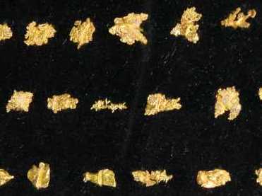
Rare dendritic formations of gold that will be analysed using the fingerprinting technique

The lab where Allen analyses the samples is fairly standard-looking - white walls, benches covered with assorted test tubes and beakers, numerous trolley-loads of interesting looking equipment. But some things are a little different. A fridge-sized safe in the corner holds over $60,000 (Australian) worth of gold, some of it incredibly beautiful and present as rare dendritic formations, awaiting analysis using the fingerprinting technique. The safe also contains an assortment of other samples to be analysed, such as gunshot residue, projectiles, glass and other metallic samples. Quietly humming in the centre of the room are several impressive-looking instruments.

The biggest of these is the Inductively Coupled Plasma Mass Spectrometer (ICP-MS), a large beige sarcophagus. Lifting the lid at one end reveals the internal workings that produce the plasma - an electrical rather than combustion flame that burns at around 8,000 degrees celsius, hotter than the centre of the earth.

The plasma is connected by a snaking tube to the Laser Ablation unit, where an ultra-violet light laser is focussed through a microscope lens onto the surface of the sample to be fingerprinted. The specific areas of the sample selected for ablation are subjected to a burst of laser light, which acts like a microscopic thermal lance, to vaporise a tiny spot on the surface just 0.02 millimetre wide.

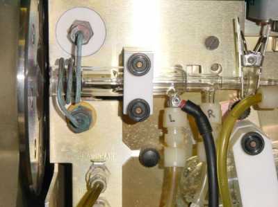
The three nested glass tubes that contain the plasma in the ICP-MS. The vaporised sample passes from the right side through the plasma and into the mass spectrometer on the left.

The vapour is drawn through the snaking tube, now filled with argon gas, into the blue plasma which causes the particles to become electrically charged. A series of electrical lenses, contained at high vacuum, guide the ions produced through the mass spectrometer, where the elements are separated according to their mass-to-charge ratio. The separated elements then smash into a detector, which keeps count of how many particles of each element pass through the instrument per second.

Laser ablation requires very little material, so the sample can be kept for future forensic examination and corroborative analysis. Sometimes, the sample to be analysed is supplied to the plasma from a solution rather than laser ablation. In this case the ICP-MS has such low detection limits that the presence of any of the elements in the periodic table can be detected in amounts of just nanograms (10^-9 grams) per kilogram - equivalent to differentiating just one grain of sand from a whole tonne of the stuff.

"The instruments have a high requirement for maintenance as the operating conditions are harsh", says Allen. "The requirement to cool the parts of the instrument which are in contact with the 8,000 degree plasma is essential to prevent the parts melting. Also, the very high vacuum requirements in the mass spectrometers require turbo-molecular pumps, which typically rotate at 100,000RPM on magnetically levitated bearings or compressed air."

Output from the ICP-MS is usually in the form of an electronic signal of counts per second for each element. These are then tabulated in a spreadsheet. However, it is not the actual values of the counts, but rather the relative intensity of each element in the sample that determines the fingerprint. The aim of the analysis, John says, is to show that some numbers are in fact relatively the same, or relatively different. For example, the numbers 153 and 260 may appear to be different to each other, but are very similar when compared to numbers such as 10,000.

But just how similar is "the same"? If the jury were presented with only this spreadsheet they would find it difficult to judge just how close two element counts need to be before they can be considered "the same". But by presenting this evidence in a visual way, focusing on the relationships between the elements in the samples, the similarities and differences between the materials analysed are much more apparent. "Juries are good at recognising patterns", says John, "so we aim to show them patterns".

One of the easiest ways to spot the patterns in the data is to produce ternary plots which emphasise how the elements in a sample are associated with one another. The relationship between three elements is plotted within an equilateral triangle whose vertices represent the three elements being considered. If there are equal amounts of each element present in a sample, it is plotted in the very centre of the triangle. If only one of the elements is present, the sample is plotted at the vertex for that element. If the sample contains only two of the three elements then it is plotted, at a point equivalent to their relative concentration, somewhere on the edge of the triangle between those two elements. Otherwise the sample is plotted somewhere in the interior of the triangle, being pulled relatively towards the vertices of the elements that dominate the sample.

A sample point on a ternary plot - marked in red

To plot a sample that when analysed produced 7000 counts of Sodium (Na) per second, 2000 counts of Iron (Fe) per second and 1000 counts of Calcium (Ca) per second, the vectors from the centre to the vertices are multiplied by the relative amounts of each of these elements in the sample and added together. Starting at the centre, we move 70% along the vector to Na, then move 20% along the arrow from the centre to Fe, and finally 10% along the arrow from the centre to Ca.

These ternary plots suggest that the three suspect samples (plotted red, yellow and green) are in fact from the same source, and unique, when compared with many samples from other sources (plotted blue)

It is the relative relationship between the counts that is important, not their actual value, so if one element is significantly larger than either or both of the other two it is possible to scale the counts in order to draw the data points into the body of the plot. Spreading the points out can make differences or similarities in the relationships clearer when comparing the samples. However, John tends to not use scaling when presenting his evidence in court, so that there is no possibility of mathematical dispersion affecting the patterns.

As samples repeatedly plot in close proximity over the different combinations of elements, it becomes more and more likely that these samples in fact come from the same source. But when can you be sure that a particular sample comes from the same source as another? Sometimes two samples may look the same when plotted using a certain three elements, but completely different when plotted against three different elements. So in order to be sure that such a case is not missed, you would need to check all possible combinations of elements in ternary plots - of which there are several thousand! - and this would take too long. So instead John first produces a "comparability index" to help him understand how similar samples are.

Plotting the raw counts per second for each element creates a spectral profile for the sample. Then you can see whether other samples are similar to the one you are trying to identify by looking at how closely their spectral profiles fit each other. The comparability index is produced by examining this degree of fit.

The sample that to be identified (called, say S1) is compared to a database of samples in which it itself (this time called S1*, say) has been included. The best fit to S1 will be S1* as the two are identical, so S1* is said to have a 100% fit. The sample that is the worst fit to S1 is taken to have a 0% fit.

But how do you determine how closely the other samples fit S1? The comparability index is a way of comparing how closely the spectral profiles of the samples in the database fit that of S1. For each sample the "difference in fit" is calculated. This is an average over all the differences in element counts from the sample in the database to S1. Logs are used to normalise out the differences. The last step is to convert all logs back to real numbers and subtract 1 to ensure that the difference of fit for S1* is 0 (the antilog of 0 is 1, since 10⁰=1).

Then the comparability value for each sample in the database can be calculated:

This calculation satisfies the requirements that the sample S1* has a comparability value of 100, while the worst match has a comparability value of 0. This comparability index produces a ranking of the samples being compared to S1 by difference of fit. It is important to remember that it doesn't provide an absolute comparison. Only the comparative rankings have significance, not the actual numbers, which in fact depend on the total number of samples in the database and the maximum difference of fit among these.

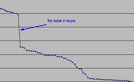
The comparability index plotted in descending order reveals the break in slope points

When the comparability values for the samples are plotted in descending order, we can detect significant changes in the slope of the graph. These turning points, or "break in slope" points, represent a change in the populations in the database (a population is a group of things with similar characteristics). Using the comparability index to sort the samples identifies those in the same population as S1. To illustrate this the spectral profiles of the samples in the same population as S1 are plotted. They usually turn out to be very close and to emphasise how similar these profiles are,. The first sample after the break in slope point is usually also plotted for comparison.

The spectral profiles for the samples in the same population as S1 appear to be very similar, whereas the profile for the first sample after the break in slope point (in dark blue) shows a marked difference

Ternary plots are then produced to show the similarities of the populations in the database, in particular between those samples in the same population as the sample being identified. It is in this final stage of interpretation of the data that the integrity of the forensic scientist is very important. Although John could choose only certain ternary plots that make particular samples look the same, he never would. In fact, he usually takes his laptop to court so that he can produce any plot that is requested there and then in the courtroom. John says that he just provides the truth as he sees it from the analysis of the sample fingerprints, and provides his interpretation and the data to both sides (the defence and prosecution) so that it can be independently verified. "You can never conclusively say that two samples are the same", he explains, "but you can provide compelling evidence to suggest that they are. You also have to give some probabilistic limits on the chance of this data occurring randomly."

At the end of the day John's job as a forensic scientist is to communicate information to the jury in a clear and unbiased way. By presenting complex scientific evidence in such a way that understanding is a more intuitive, natural process, John and Allen are helping to better prepare jurors for making their final judgements.

About this article

Rachel Thomas is assistant editor on Plus. For this article Rachel interviewed John Watling and Allen Thomas from Curtin University's School of Applied Chemistry in Western Australia.

John Watling is Associate Professor in Forensic Chemistry in the Applied Chemistry School at Curtin University of Technology. He has a lifetime of experience in Analytical and Applied Chemistry, and is also a Chartered Analytical Chemist. He has served as expert witness in very many court cases worldwide. One of his major interests is using fingerprinting techniques to provenance precious metals, diamonds and other precious stones; and in detecting fraud in works of art and antiquities. Another is scene-of-crime analysis and characterisation. John has been instrumental in establishing a worldwide network in Forensic Criminalistics.

Allen Thomas is an Analytical Chemist with a strong interest in the application of computer science to characterisation and pattern recognition for interpretation of analytical data. He has developed software for graphical display of data to aid in pattern recognition and fingerprinting.