Knowing when to quit

Knowing when to quit is one of life's great dilemmas, whether to persist in the face of diminishing rewards, or to quit now in the hope of finding richer rewards further afield. For every gold mine, eventually there comes a point when the amount of gold extracted can no longer justify the cost of keeping the mine open; once that point has been reached, it is time to quit, and start looking for a new mine.

Similarly, for a bird feeding on caterpillars in a bush, there comes a point when the calories gained can no longer justify the energy expended in searching for more caterpillars; once that point has been reached, it is time to quit, and move to another bush. And, for a honeybee, there comes a time when the weight of pollen collected can no longer justify the energy required to carry that pollen; at that point it is time to quit collecting, and fly back to the hive.

Fortunately, there is a mathematical recipe, embodied in the marginal value theorem (developed by the American ecologist Eric Charnov in 1976), which specifies when to quit in order to maximise rewards. More importantly, the marginal value theorem has an enormously wide range of applications, from its origins in optimal foraging theory to how brains process information. In essence, the marginal value theorem provides a general strategy for maximising the bang per buck, irrespective of the nature of the bang and the buck under consideration.

She doesn't have far to look for her next meal (Image Greyson Orlando – CC BY-SA 3.0)

Ladybirds on the hunt

Ladybirds feed on aphids, but watching a ladybird eating an aphid is like watching a human eating a lobster, because the aphid's exoskeleton is as impenetrable to a ladybird as the lobster's exoskeleton is to a human. In both cases, after an initial flurry of activity during which the juiciest parts are eaten, increasing amounts of effort are required to extract decreasing amounts of food. The dilemma faced by the human is knowing when to quit and move on to another dish. Similarly the dilemma faced by the ladybird is knowing when to quit, and go in search of another aphid.

If the ladybird quits feeding on an aphid too soon then she wastes food that is easily accessible. Alternatively, if she quits too late then increasing amounts of effort are required to obtain diminishing amounts of food, which might otherwise be obtained easily by finding another aphid. Clearly, there is an optimal "Goldilocks time" to quit; a time that is neither too soon nor too late. To work out when this Goldilocks time has arrived, we need to examine the eating behaviour of ladybirds in more detail.

The lobster-like nature of aphid anatomy means that, if a ladybird is left alone to feed on an aphid then the cumulative weight of food eaten increases with feeding time $t$ in a manner shown by the data points below. (The data is from a classic paper on optimal foraging theory by RM Cook and BJ Cockrell published in 1978, which inspired our ladybird example.)

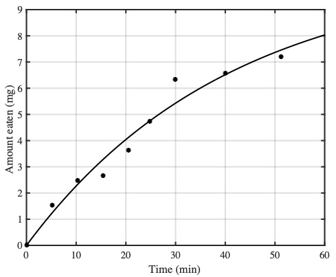
$The weight of tissue eaten (black dots) from an aphid in $t$ minutes, fitted with a \emph{reward function} $E(t)$ (black curve).$

The weight of tissue eaten (black dots) from an aphid in t minutes, fitted with a reward function, E(t) (black curve).

These data points can be fitted with with a reward function $E(t)$ , described by the curve $E(t)=a(1-e^{-bt})$ , where $a=10.43, b=0.0245$ for our ladybird example. We can use this reward function to define two key quantities:

The instantaneous reward rate, $r(t) = \Delta E(t)/\Delta t$ , which is the number $\Delta E(t)$ of calories gained per time period $\Delta t$ (eg. calories gained per minute).
The running average reward rate, $R(t)=E(t)/(T+t)$ . This is the cumulative weight of food eaten after feeding on an aphid for $t$ minutes, divided by the search time $T$ taken to find this aphid plus the time $t$ spent feeding on this aphid.

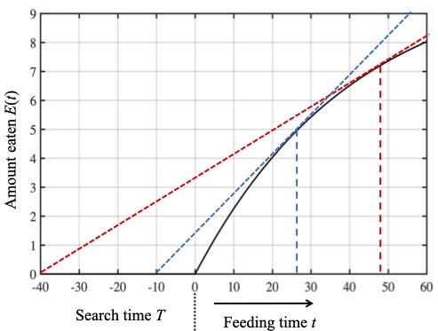
These quantities have reasonably intuitive geometric interpretations. The figures below use the reward function fitted to the ladybird data above, to show the accumulated amount of reward $E(t)$ after a food source is found in time $T$ .

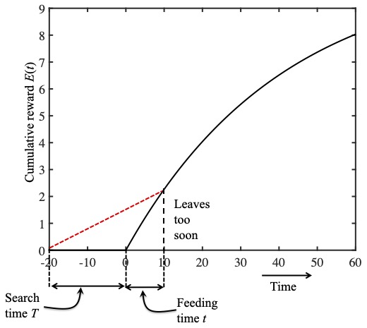
The black curve in these figures is the reward function $E(t)$. The slope of this curve is the reward per minute in the past minute: instantaneous reward rate $r(t)$.

The black curve in these figures is the reward function E(t) and the slope of this curve is the instantaneous reward rate r(t). The slope of the dashed red line is the average reward rate R(t). In this figure the ladybird leaves too soon.

At a point $t$ after the aphid is found, we can define a right-angled triangle with a base of length $T+t$ , and height $E(t)$ (the dashed black vertical line). The third side of this right-angled triangle is the red dashed red line, and the slope of this line is equal to $E(t)/(T+t)$ : the running average reward rate $R(t)$ . This means we can express the problem of maximising the running average reward rate in terms of the slope of the red dashed line. Specifically, which red dashed line has the largest possible slope?

In the top figure to the right, a feeding time of $t=10$ minutes yields a small slope which would be larger if the ladybird quit feeding later: she left too soon and her running average reward rate would be larger if she fed for more than 10 minutes.

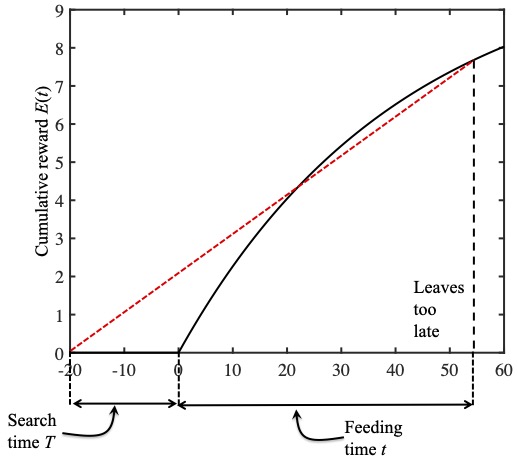
In this middle figure the ladybird leaves to late.

Similarly, in the figure in the middle , a feeding time of $t=55$ minutes also yields a small slope; which would be larger if she quit feeding sooner. She left too late and her running average reward rate would be larger if she fed for less than 55 minutes.

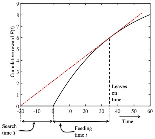
In this figure the ladybird leaves at just the right time.

Finally, in bottom figure, a feeding time of $t=35$ minutes yields a the largest possible slope; this is the optimal time to feed as her running average reward rate would be maximal if she were to quit feeding after 35 minutes.

Notice that this Goldilocks feeding time occurs after feeding for a time $t$ when the slope $r(t)$ of the reward function exactly matches the slope of the red dashed line, which is equal to the running average reward rate $R(t)$ . In other words, the Goldilocks feeding time occurs after feeding for a time $t$ when the running average reward rate equals the instantaneous reward rate: $r(t)=R(t)$ .

As a geometric confirmation, the instantaneous reward rate $r(t)$ is plotted as a red dashed curve in the figure below, and the average running reward rate $R(t)$ is plotted as a black solid curve.

As a geometric confirmation, the instantaneous reward rate $r(t)$ is plotted as a red dashed curve in the figure above, and the average running reward rate $R(t)$ is plotted as a black solid curve.

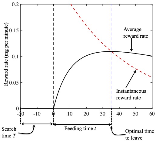
The instantaneous reward rate r(t) is plotted as a red dashed curve in the figure above, and the average running reward rate R(t) is plotted as a black solid curve.

As we should now expect, these two curves cross at the Goldilocks quitting time (i.e. where $r(t)=R(t)$ ). This geometric analysis has effectively proved the marginal value theorem, which states that the optimal time to quit is when the instantaneous reward rate equals the running average reward rate; that is, when $r(t)=R(t)$ . (You can see a mathematical proof of the marginal value theorem here.)

Ladybirds know the marginal value theorem

The above analysis assumed a constant search time $T$ . But a proper test of the predictions of the marginal value theorem would also involve varying search times. In essence, long search times suggest food is scarce, so it makes sense to increase the time spent feeding on each aphid accordingly. In other words, the amount of time spent feeding on a particular aphid should increase with the time taken to find that aphid. However, beyond this correct but vague conclusion, the marginal value theorem predicts precisely how much feeding time should increase with search time, as shown in the figure below (again using the reward function based on data from Cook and Cockrell’s experiments in 1978).

If it takes 40 minutes to find an aphid then the ladybird should spend about 50 minutes feeding on that aphid (red dashed line), but if it only takes 10 minutes to find an aphid then the ladybird should spend only about 28 minutes feeding (the blue dashed line).

We can see from this figure that the marginal value theorem predicts that time spent feeding on an aphid increases with the time taken to find that aphid. If it takes 40 minutes to find an aphid then the ladybird should spend about 50 minutes feeding on that aphid (the red dashed line in the figure above). If it takes 10 minutes to find an aphid then the ladybird should spend only about 28 minutes feeding (the blue dashed line).

The question is, do ladybirds quit in accordance with the predictions of the marginal value theorem? To answer this question, Cook and Cockrell scattered aphids around at random on a tray, and then measured the time $T$ taken for ladybird larvae to find each aphid, and the time $t$ spent feeding on each aphid. (Cook and Cockrell used ladybird larvae rather than ladybirds, but that does not matter here).

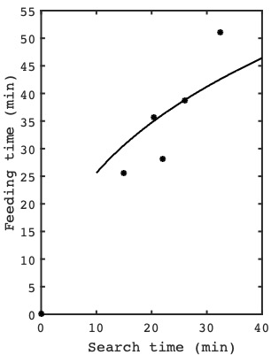
The average feeding time Cook and Cockrell observed for the ladybird larvae observed, as it varied with search time: the dots represent observations from their experiments and the black curve is the feeding times predicted by the marginal value theorem.

How the average feeding time of the ladybird larvae varies with the search time required to find an aphid: the dots represent observations from experiments and the black curve is the feeding times predicted by the marginal value theorem.

The plot on the right shows how the average time spent feeding for the ladybird larvae observed by Cook and Cockrell varied with search time: the dots represent observations from their experiments and the black curve is the feeding times predicted by the marginal value theorem. Over many experiments, the number of aphids was gradually decreased, which increased search times accordingly. As predicted, the average time spent feeding on each aphid increased as search times increased (i.e. as the density of aphids decreased). More importantly, the average time spent feeding on each aphid increased with search times in a manner consistent with the marginal value theorem, as shown in figure above.

In this particular example, the fit between the data and theory is not impressive. This may be because the running average reward rate function $R(t)$ does not have a sharp peak, so the efficiency penalty for quitting a little early or late is relatively small. In contrast, if the reward function rises more steeply then the running average reward rate has a higher peak and it’s more likely that the experimental data would be a closer match to the predictions of the marginal value theorem.

Animals know when to quit

The way that ladybirds hunt for aphids is just one of many examples of how animals maximise food intake by quitting at just the right time. But the same lessons can be applied to any situation in which acquiring a valuable resource is costly.

The great minds of great tits

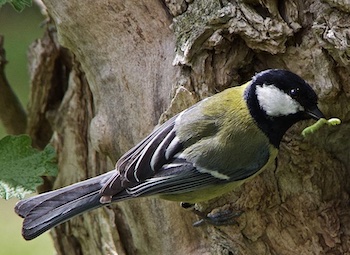
(Image by resembler – CC BY-SA 4.0)

Consider a great tit that has spent some time searching for a bush that contains an abundance of caterpillars. Having found a bush, the great tit initially eats a large number of caterpillars per minute, but after a little while, the number of caterpillars available decreases, so the number of caterpillars eaten per minute falls. Given these diminishing returns, when should the great tit quit this bush, and search for another bush of caterpillars?

As was the case for the ladybird example above, the answer is provided by the marginal value theorem. By running experiments analogous to the ladybird experiments described above, the scientist Richard Cowie observed in 1977 that the quitting times of great tits was correctly predicted by the marginal value theorem.

Quitting sex

For a male dungfly, knowing how long to mate with a female dungfly represents a classic trade-off between the lure of a guaranteed immediate reward and an uncertain, but possibly larger, future reward. The longer a male mates with a female the more sperm from previous matings by other males can be displaced, and the less opportunity the female has to mate with other males. But every minute a male spends mating with a female is a minute he could have spent mating with other females.

Notice that the time taken to find a new female corresponds to the time required to find a new food source (a new aphid or a new bush) in the previous examples, and that the time spent mating with one female corresponds to an increasing, but diminishing, reward. Accordingly, we should not be surprised to learn that the marginal value theorem predicts just how long a male dungfly should mate with each female to ensure that he has as many offspring from as many females as possible. In 1976, the scientists G.A. Parker and R. A. Stuart observed that male dungflies spend an average of 36 minutes mating with each female, which is comparable to 41 minutes predicted by the marginal value theorem.

Are bees too busy to be efficient?

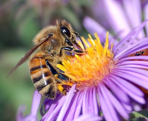
As a honeybee collects more pollen, the amount of energy expended carrying the pollen back to the hive increases. The dilemma faced by every honeybee is this: At what point should the honeybee quit collecting pollen and return to the hive?

At one extreme, if the honeybee returns after collecting a single grain of pollen then the energy used in flying to and from the hive almost certainly exceeds the energy obtained from the pollen grain. At the other extreme, if the honeybee collects a large load of pollen then the rate at which pollen is collected will be large, but the energy expended in flying back to the hive could be a substantial proportion of the energy obtained from the pollen. Between these two extremes is a Goldilocks load size which provides the maximum possible pollen energy gained for each calorie expended in flying. Notice that there are diminishing returns because the honeybee's load increases with each successive flower visited.

Using a range of distances between the hive and flowers, the scientists Paul Schmid-Hempel, Alejandro Kacelnik and Alasdair Houston observed in experiments in 1985 that the pollen loads carried by honeybees matched those predicted by the marginal value theorem. In short, honeybees collect pollen as efficiently as possible in terms of the energy expended per gram of pollen collected. In contrast, a model based on maximising the rate at which pollen was collected per minute yielded a very poor fit to the pollen loads, suggesting that honeybees favour energy efficiency over the rate of pollen collection.

Brains and the marginal value theorem

Neurons process information, and that is pretty much all they do. But neurons are extremely expensive to maintain, and even more expensive to use to transmit information, so it makes sense that they should run at maximum efficiency.

According to Claude Shannon's theory of information, a convenient unit of information is the bit, which provides enough information to choose between two equally likely alternatives (like the flipping of a coin). However, Shannon's theory defines a universal law of diminishing returns, which means that the energy required to process each bit of information increases with the number of bits processed per second. Consequently, information can be processed cheaply at low rates, or expensively at high rates, but it cannot be processed cheaply at high rates.

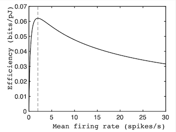
How energy efficiency varies with firing rate for neurons. The peak of this curve correctly predicts the average firing rates of neurons, which is consistent with the idea that neurons maximise energy efficiency (pJ stands for pico-Joule).

Notice that this law of diminishing returns is analogous to the problem that confronts the ladybird, where there are diminishing returns for the amount of food eaten per second. The difference is that, whereas a ladybird wants to maximise the average amount of food eaten per second, a neuron wants to maximise the average amount of information it processes per Joule of energy expended. Given these similarities, we should not be surprised to find that the ladybird's problem and the neuron's problem can both be solved using the marginal value theorem.

Consequently, the marginal value theorem can be re-cast in terms of energy expended (which replaces time) and information (which acts as the reward). The resultant efficiency curve shows that the maximum efficiency (measured in bits/Joule) predicted by the marginal value theorem occurs at a firing rate of about 2 neuronal spikes per second. Crucially, in 1996 the scientists William Levy and Robert Baxter found that this prediction agrees with their observations of the average of firing rate of neurons.

Thus, the marginal value theorem specifies how much to pay to maximise rewards, whether payment is measured in time spent searching for aphids or energy expended in neuronal spikes, and whether reward is measured in aphids eaten per hour, or bits of information processed per Joule.

About this article

James V. Stone is an Honorary Associate Professor at the University of Sheffield, England. He would like to thank John Frisby, Nikki Hunkin and Raymond Lister for their comments on this article.

Comments

correct link

The correct link to James Stone's books is here:
https://jamesstone.sites.sheffield.ac.uk/books

Plus.Maths.org