Model Trains
Going Places with Maths
If you ask anyone what they dislike about trains, the chances are they will say one of two things: "They're always late" or "They're too crowded". As it happens, both of these problems have been studied using mathematical modelling techniques. This article looks at the latter problem, a topic known as "Peak Load Management".
An unusual sight on our railways...
©trainweb.com
The problem of predicting train loads (though not always reducing crowding!) has been successfully tackled by mathematicians working as consultants within the rail industry. This article will also give a feel for the techniques and approaches used by such consultants, which is highly representative of the way mathematics is used in real-life.
To start thinking about this problem, we will first need a clear definition, something better than "They're too crowded"! Getting to the first definition should be simple:
At certain times of the day, trains become very crowded, due to people wanting to travel to and from work.
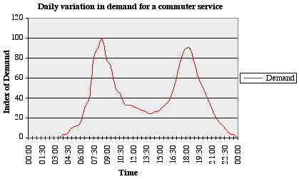
The diagram below shows how demand for a commuter train service typically varies during the day. Peak Load Management is about trying to cope with this changing demand, without trains becoming too overcrowded.
Fine, but we need to understand exactly what the consultant is required to do about it! Here is a more thorough definition of the problem:
- Trains are crowded at peak times. This causes dissatisfaction amongst passengers, and may lead to fewer people using the trains.
- Train timetables are complicated - it is difficult to know which trains people will prefer, or if the right amount of rolling stock is currently being used for each route. Lengths of trains, frequency and stopping patterns can all be altered.
- It is even more difficult to know how people will behave when changes are made to the timetable or rolling stock. For example, is it better to introduce more frequent, smaller trains, or to make current trains longer?
- If more rolling stock is to be used, then a firm prediction must be made of how much is needed. Having too much wastes money, having too little drives customers away.
How Mathematics can help
Mathematical modelling has been used to tackle this problem for many years, and a core approach is well established. However, in each project there are interesting variations, depending on the client's precise needs. In this article we'll look at a generic outline of how the mathematical model is built up, covering both the basic principles and some special cases from recent projects.
There are three basic stages:
- Understanding the choices customers are making at present;
- Building models which can help understand future choices;
- Using the model to produce results meaningful to the client.
1. Understanding current choices
There is a mathematical model which has been used for many years to model customer behaviour. Let's look at the factors that such a model would have to include.Thinking about customer choices
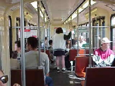
Getting from A to B.
©trainweb.com
If we think simply about the choices passengers must make, then it is clear that each customer wishes to get from a point A to a point B. Customers want to do this in the shortest amount of time possible, and to arrive at the time that suits them. They may also have some preferences about the type of train they travel on; for example, regular travellers may prefer to avoid certain very crowded trains.
Since the ideal journey would be one that took no time at all, and every other journey of course falls short of this ideal, we can think of the problem as a minimisation problem. Each customer tries to minimise some combination of the inevitable (at least until train companies utilise teleport technology!) real-world inconveniences of travel. We'll call this combination the attractiveness of a train to a customer who can choose between a number of different trains.
The first factor to take into account in describing this attractiveness is the length of time the journey takes. If this were the only factor, we could write $$A_{C,T} = t_{C,T},$$ where $A_{C,T}$ is the attractiveness of train T for customer C, and $t_{C,T}$ is the journey time on train T of the journey customer C wishes to make.
This first attempt is very crude, but we can improve it by also taking into account the difference between the time the customer wanted to arrive at, and the actual arrival time of the train: $$A_{C,T} = t_{C,T} - N(a_T - d_C),$$ where $a_T$ is the actual arrival time on train $T$, $d_C$ is the time the customer would have liked to arrive at, and $N$ is a number telling us how much better or worse it is to be an extra minute early or late, compared with an extra minute spent travelling.
This equation means that the attractiveness of a train arriving exactly at the desired arrival time equals the travel time. For a train arriving 5 minutes before or after the desired arrival time, there is a further penalty of $5 \times N$. \par The final factor we will take into account is the crowding on the train. We modify the equation further, to get $$A_{C,T} = \left[ t_{C,T} - N(a_T - d_C) \right] \times f\left(l_T/c_T \right),$$ where $l_T$ is the trainload, $c_T$ is the number of seats on the train, and $f$ is a factor describing the importance of crowding.
When this equation is used to describe the attractiveness of trains, the result looks something like the diagram below. Because of its appearance, this is called a "rooftop chart".
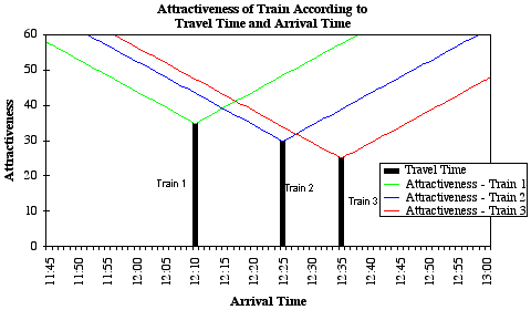
For a customer with a given arrival time, the attractiveness of a train is equal to the travel time, plus an allowance for the distance from their preferred arrival time. Using the graph, this means finding the train with the smallest attractiveness value at the customer's preferred arrival time. (Remember, as journey time increases, so does attractiveness. This means the trains become more "attractive" to customers as our attractiveness measure decreases.) For someone wanting to arrive at 12:15, Train 1 and Train 2 are equally attractive. Any earlier, and Train 1 becomes more attractive, any later and Train 2 wins.
In this way, we can begin to reason about how people make choices between trains. The approach can be revised as needed when we wish to look at other issues, such as level of crowding, or if we wish to take into account, say, departure rather than arrival time.
Studying data on customer behaviour
What I have described above is model-building largely by common sense and conjecture. The real effort goes into testing these hypotheses and calculating the true values of parameters such as N. We will not describe this process in detail, but here is an overview of how it works:
- Actual data on numbers of people travelling are collected.
- Cases where just one factor has changed in isolation are found (say, one train arrives 10 minutes later than previously, all the others stay the same).
- The numbers choosing that train before and after the change are analysed to find a value for the factor N.
Whole essays could be written on the approaches used to find different factors, either in isolation or experimentation. The techniques might involve interviewing customers to assess their stated preferences for different options (for example, a fast, infrequent service, versus a slow frequent service), or analysing very large amounts of historic data to assess whether the effects are truly linear (as assumed here) or whether more complex equations should be used.
2. Building a model
Once equations have been arrived at to explain customer choices, we are ready to build a model. This will allow us to think about what might happen to customer behaviour, and hence train loadings, if :- Demand increases (or decreases!);
- The timetable changes (more trains, faster trains);
- The number of seats available changes (longer trains).
We'll look in detail at a simple case where there are only six trains, and only one origin and destination point. Obviously, in reality the situation would be much more complex, with trains calling at many points along the route. However, this simple example illustrates the general procedure.
The demand profile
First of all we need to quantify when people want to travel. We do this by splitting the time we want to study into time bands. In this case we are looking at a morning peak period, and the time is split into ten-minute bands, as shown in the table below:
|
|
|
We should ideally include the capacity of the trains and look at crowding, but for simplicity we'll leave that out for now.
Choosing the best train
Now, we simply apply the equation to see which train is most attractive in each time band. The table below shows the attractiveness values for each train and departure time, using a value of 0.5 for N. Remember that the lower the attractiveness value, the more attractive the train.| Time | Train 1 | Train 2 | Train 3 | Train 4 | Train 5 | Train 6 | Minimum | Best Train |
|---|---|---|---|---|---|---|---|---|
| 7:00 | 30.0 | 42.5 | 65.0 | 70.0 | 80.0 | 90.0 | 30.0 | Train 1 |
| 7:10 | 25.0 | 37.5 | 60.0 | 65.0 | 75.0 | 85.0 | 25.0 | Train 1 |
| 7:20 | 20.0 | 32.5 | 55.0 | 60.0 | 70.0 | 80.0 | 20.0 | Train 1 |
| 7:30 | 15.0 | 27.5 | 50.0 | 55.0 | 65.0 | 75.0 | 15.0 | Train 1 |
| 7:40 | 20.0 | 22.5 | 45.0 | 50.0 | 60.0 | 70.0 | 20.0 | Train 1 |
| 7:50 | 25.0 | 22.5 | 40.0 | 45.0 | 55.0 | 65.0 | 22.5 | Train 2 |
| 8:00 | 30.0 | 27.5 | 35.0 | 40.0 | 50.0 | 60.0 | 27.5 | Train 2 |
| 8:10 | 35.0 | 32.5 | 30.0 | 35.0 | 45.0 | 55.0 | 30.0 | Train 3 |
| 8:20 | 40.0 | 37.5 | 25.0 | 30.0 | 40.0 | 50.0 | 25.0 | Train 3 |
| 8:30 | 45.0 | 42.5 | 30.0 | 25.0 | 35.0 | 45.0 | 25.0 | Train 4 |
| 8:40 | 50.0 | 47.5 | 35.0 | 30.0 | 30.0 | 40.0 | 30.0 | Train 4 |
| 8:50 | 55.0 | 52.5 | 40.0 | 35.0 | 25.0 | 35.0 | 25.0 | Train 5 |
| 9:00 | 60.0 | 57.5 | 45.0 | 40.0 | 20.0 | 30.0 | 20.0 | Train 5 |
| 9:10 | 65.0 | 62.5 | 50.0 | 45.0 | 25.0 | 25.0 | 25.0 | Train 5 |
| 9:20 | 70.0 | 67.5 | 55.0 | 50.0 | 30.0 | 20.0 | 20.0 | Train 6 |
| 9:30 | 75.0 | 72.5 | 60.0 | 55.0 | 35.0 | 15.0 | 15.0 | Train 6 |
| 9:40 | 80.0 | 77.5 | 65.0 | 60.0 | 40.0 | 20.0 | 20.0 | Train 6 |
| 9:50 | 85.0 | 82.5 | 70.0 | 65.0 | 45.0 | 25.0 | 25.0 | Train 6 |
| 10:00 | 90.0 | 87.5 | 75.0 | 70.0 | 50.0 | 30.0 | 30.0 | Train 6 |
Allocating Demand to Trains
Since this is a simple model we'll assume that everyone boards the best train (in real models we assume some people board the second and third best trains, which does in fact happen in reality. This is sometimes referred to as a "fuzzy logic" approach). This gives the following train loads:| Train 1 | Train 2 | Train 3 | Train 4 | Train 5 | Train 6 | |
|---|---|---|---|---|---|---|
| Total Load | 151 | 159 | 207 | 199 | 187 | 97 |
This is the model in a nutshell. Now we can change the number of trains, the train times, the demand level or the demand profile and instantly see the effect.
Looking at model accuracy
The model can now help us understand how passengers might behave, but we can never be certain the model is correct. We are talking about real people after all, and their precise behaviour is hard to predict! However, in business it is useful to be able to reassure the client that the model's predictions are "good enough" for their purposes.
In this case, three areas can be considered to see how good the prediction is:
- We may not have predicted overall future demand correctly. We may be predicting a 10% increase in customers, but what if it turns out to be 12%, or only 8%? This can have a major impact on the decisions made.
- The model might not properly predict how customers respond to longer or more frequent trains. What if the value of N should be 0.4 or 0.6 rather than 0.5?
- Customer behaviour might vary from day to day, and we may require a result which takes this into account.
The first two of these might be tackled by what is known as "sensitivity analysis". This usually involves entering various values of demand, say, into the model and recording how much the answer changes. We might also analyse input data to assess how likely it is that the value of N or the demand prediction should change. Combining this, we can usually advise the client on a number of higher and lower "scenarios" and the likelihood of each of these.
The final case is dealt with in the section below.
3. Producing meaningful results for clients
Having the model isn't everything. We must understand the results it gives well enough to advise clients. In a recent piece of work a client was specifically interested in the number of passengers who would be standing on trains when a new timetable was introduced.When considering numbers standing, we found that statistical analysis of the model results was required to provide meaningful figures. To see why, consider the predictions of numbers standing produced in our example above:| Train 1 | Train 2 | Train 3 | Train 4 | Train 5 | Train 6 | |
|---|---|---|---|---|---|---|
| Total Load | 151 | 159 | 207 | 199 | 187 | 97 |
| Capacity | 100 | 160 | 160 | 160 | 160 | 100 |
| Standing | 51 | 0 | 47 | 39 | 27 | 0 |
So the model predicts a total of 164 people standing. However, what if this predicted load is the average for the year, and the number of passengers varies from day to day? For example, Train 2 could have 0 people standing on an average day, but on a "bad day" there would be some standing. The results sent to the client needed to reflect this.
The important point was to understand how much train loads vary, and find a way to take account of this. We can use statistical methods to analyse historic data and describe the variation. This will allow us to estimate numbers standing on average.
Typically, train loads vary as shown in the diagram below.
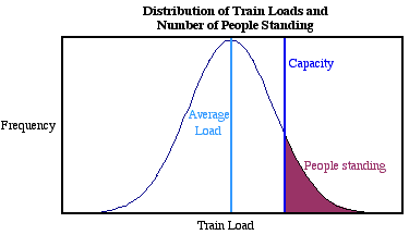
The dark blue line marks the capacity of the train - so if there are more people on the train, the extra must stand. Notice that most trains carry around the average number of passengers - only a few carry far more or far fewer than that average. If you know a little about integration you will see that the shaded area on the diagram represents the average number of people standing on a given day.
This sort of distribution is called the normal distribution - so-called because it appears so often when random variations are studied that it is the "normal" thing to see! A lot is known about this distribution - in particular we can integrate to find the shaded area. Doing this, we can get a more accurate estimate of number of people standing. Here is the result:
| Train 1 | Train 2 | Train 3 | Train 4 | Train 5 | Train 6 | |
|---|---|---|---|---|---|---|
| Total Load | 151 | 159 | 207 | 199 | 187 | 97 |
| Capacity | 100 | 160 | 160 | 160 | 160 | 100 |
| Numbers standing (model) |
51 | 0 | 47 | 39 | 27 | 0 |
| Numbers standing (inc. random fluctuations) |
52 | 12 | 48 | 40 | 30 | 12 |
So in fact, all of the trains will have some standing, on certain days. The model has initially assumed that every day is the same, and that the actual number of people standing on any given day is the same as the average number standing on all days. As we have seen, random fluctuations in passenger numbers means that this won't be so.
Mathematics - How it really is
Using mathematics in "real" business applications is different from studying or using mathematics in an academic environment. Clients are interested primarily in the "bottom line", which requires the consultant to be highly focused on immediate goals - goals which are defined by a client or a business. The nature of proof is also different: in business, mathematics needs to be seen to deliver results to the satisfaction of the client. We must be confident of usefulness and applicability of the results, but a rigorous mathematical proof is unlikely to be required. Rather than striving to understand everything about a subject, we usually seek to know "just enough" to produce a solution which is "good enough".
Using mathematics in a business environment provides some unique problems that aren't encountered in academia. There is the difficult task of understanding the client's problem. Then there is the task of finding established techniques to help or very often developing new approaches. One of the chief joys of working in a business environment is that nearly every problem is different and requires a fresh approach. This means the consultant is constantly called on to think creatively and challenged to innovate, with every solution being tested in the real world.
This is all part of a mathematical discipline called "Operational Research", which is used in business, industry, government and military applications. Techniques used are very varied, including statistical analysis, computer modelling or informal analysis and advice to clients. Applications in the rail industry are similarly varied: in addition to peak load management, mathematics has assisted in analysis the causes of delays, building timetables, advising on how to maximise revenue, and dozens of other applications.
About the author
 Tim took a degree in Mathematics before studying for an MSc in Operational Research at Lancaster University. He subsequently worked in a range of Operational Research roles in industry, including Post Office Counters, where he worked on Network Strategy and Geographical Information Systems, and Thames Water, where he developed computer models simulating the
water treatment process.
Tim took a degree in Mathematics before studying for an MSc in Operational Research at Lancaster University. He subsequently worked in a range of Operational Research roles in industry, including Post Office Counters, where he worked on Network Strategy and Geographical Information Systems, and Thames Water, where he developed computer models simulating the
water treatment process.
Tim moved to AEA Technology Rail in 1999, where he runs the Load Management Service, and takes part in a wide range of rail service development projects for train operators.