Backgammon: the game

Backgammon is said to be one of the oldest games in the world. Its roots may well reach back 5,000 years, into the former Mesopotamia. From there, it spread out in variants to Greece and Rome as well as to India and China. It was played in England in 1743 when Edmond Hoyle fixed the rules for backgammon in Europe. After a revision in 1931 in the US, these rules are still in use today.

What turned it into the subtle and skilful game we know today was a brilliant innovation in the rules early in the 20th century: the doubling cube. Who invented it is unknown, but it emerged in American gambling clubs some time in the 1920s. In this article we'll look at some of the properties of the doubling cube.

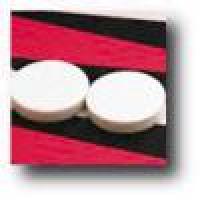
Backgammon board and some checkers

Backgammon is a game of chance and skill. It is played by two players with 15 checkers each - one player plays black, the other white. The players' checkers move in opposite directions on a board with 24 spaces.

Each player's goal is to be the first to bring all their own checkers "home" (into their own quarter of the board) and then "bear them off" (remove them from the board altogether). The movement of the checkers follows the outcome of a roll of two dice, the numbers on the two dice constituting separate moves. For the rules of the game see, for example, <http://www.bkgm.com>.

Backgammon is a gambling game, like poker, say. It has an element of chance (introduced by the dice), and there is a notion of the stake for which the players are playing. (Of course, this does not have to be actual money; in a tournament it could be points, for example.) The actual amount that changes hands can be more than the stake, however. For instance, in certain winning positions called gammon and backgammon, the stake is doubled or trebled, respectively. The other way the stake can change is by means of the doubling cube.

The Doubling Cube

If one of the players thinks that she is in the position to win the game, she can turn the doubling cube and announce a double, which means that the total stake will be doubled. If her opponent refuses the double, he immediately loses his (undoubled) stake and the game is finished. If he accepts the double, the stakes are doubled and, as a compensation, the doubling cube is handed over to him and he gets the exclusive right to announce the next double. (He is now said to own the cube.) If the luck of the game changes so that he later judges that he is now winning, he will be in a position to announce a so-called redouble, which means that the stake is doubled again. If the first player refuses the double, she now loses the doubled stake; if she accepts, the game goes on with a redoubled stake, four times the original value.

There is no limit to how many times the stake can be doubled, but the right to announce a double switches from one player to the other every time it is exercised. (Initially either player can double - no-one owns the cube.) This nice subtlety leads to a variety of tactical possibilities and problems. In this article we'll look at this element of the game from a mathematical point of view.

A doubling strategy is given by a pair of probabilities and , with . If your chances of winning reach the (high) level then, as long as your opponent doesn't own the cube, you announce a double. However, if your opponent announces a double, you accept it so long as your chances of winning are at least the (lower) amount . We would like to find optimal values for and - that is, values which maximise a player's expected winnings.

To do this we will use Brownian motion to model the evolution of Player A's chance of winning.

A Mathematical Model of the Game

Of course, we can't give a neat mathematical model for the board-play, taking account of all possible positions and dice-rolls, in this article (or at all!). Our aim is more modest, namely to model the way the game is affected by the doubling cube. To do this we will assume that we are advising an experienced player who is an expert in the board-play, and is able to make a good estimate of her probability of winning at each stage in the game. We'll base our advice about handling the cube on just this single number between 0 and 1 - or 0% and 100% if you prefer.

As the game progresses, the player's estimate of her winning chances will undergo constant revision with each successive dice-roll. We will consider the evolution of the winning chances of Player A as a time-dependent process (technically called a stochastic process) taking values between 0 and 1. To make it easier for us to model the game effectively, this process should, as a minimum, satisfy the following conditions:

Rules for the evolution of chances

1. Whether the winning chances of Player A increase or decrease after the next move is independent of the previous moves. This is natural, because rolls of the dice do not affect each other.
2. Observe that Player A wins the game exactly if her chance of winning reaches 1 (certainty) before it falls down to 0 (no chance at all). Hence the process we use to to model the game should be stopped as soon as it reaches either 0 or 1.
3. The evolution of the winning chances should be fair in some sense: in some (small) time interval, Player A's chances should be equally likely to go up by a certain amount as to go down by the same amount.
4. The process should be consistent. This means, for instance, that if the chances of Player A at a certain time are equal to 0.8, say, then the process should eventually hit the value 1 with probability 0.8 and, conversely, reach the value 0 with probability 0.2.
5. The process should be continuous. This is a mathematical idealization corresponding to the fact that with each move the chances only change a little. When treating problems like this mathematically, it is a huge convenience to look at the process in continuous time.

It's worth noting that this last assumption is a very big one. In real life, Player A's winning chances jump by a discrete amount every time the dice are rolled. However, early in the game, the jumps are usually quite small, so this assumption of continuity - which simplifies the analysis - will be fairly close to the truth. (On the other hand, later on, for instance when there are only a few checkers left in play, one particularly good or bad roll can change a player's chances from 90% to 0%, so our results will be less useful at this stage of the game.)

Can we hope to find a mathematical model (in other words a stochastic process) satisfying these conditions? The answer to this question is yes and the model that works has a long and interesting history.

In 1828, the British botanist Robert Brown studied the random motion of small pollen particles on the surface of water. This random motion is due to the fact that small particles (that is, water molecules) hit the pollen randomly.

A random walk R

If we only look at vertical movements we are in a one-dimensional situation. Whenever a particle of pollen is hit from above by a molecule it moves downwards and vice versa, as in the figure to the left.

The rules describing this random motion are pretty similar to the rules we have formulated for our evolution of chances above: After each roll of the dice, your winning chances are "hit" from above or below and therefore rise or fall by a certain random value, in a way that is independent of what has gone before. A first model of our random process therefore would be given by a stopped random walk which starts at 0.5 and jumps after each roll of dice by an independent randomly distributed value. It is stopped once it falls below 0 or rises above 1. We call the first time that either of these events happens the stopping time.

If we take into account that there are many such steps and that, as we have seen, your chances often change only a little after each roll, it is natural to ask whether there is a continuous analogue of this process. Luckily, there is such a limit. Just keep choosing smaller and smaller step-sizes for the random walk. Of course the increments of the random walk in each step are getting smaller as well. As the step-sizes get closer and closer to zero, the random walk looks more and more like a continuous-time process, called Brownian motion in probability theory.

Brownian motion was first studied as a mathematical object by Bachelier (1900) in the theory of stock markets and by Einstein (1905) to verify the molecular theory of heat. These two authors also conjectured many of the properties of Brownian motion. But it took some time to prove that Brownian motion really exists - an American mathematician called Wiener finally succeeded in 1923. The reason it isn't obvious is that you have to check that the properties required of such an object don't contradict each other. Much later (in 1951) Donsker gave a full proof of the convergence of random walks to Brownian motion. The picture to the right shows the paths of a typical random walk and a limiting Brownian motion.

A random walk (left), and limiting Brownian motion

Brownian motion appears in an extraordinary number of places - it plays a crucial role in physics (think of diffusion of particles and heat conduction) as well as in the theory of finance (think of the stock price as a small particle which is "hit" by buyers and sellers: it rises when hit by a buyer and falls when hit by a seller). Its exciting properties are widely studied by mathematicians. For example, one interesting feature is that it is nowhere differentiable (although it is continuous!) - this indicates some kind of fractal structure of its paths.

For our purposes, it is good enough to know that Brownian motion exists - that we can assume our properties (1)-(5) without some subtle contradiction appearing - and that it is indeed the limit of random walks, such as that of Player A's chances of winning under the influence of the dice, with small increments. So a Brownian motion started at 1/2, and stopped when it hits 0 or 1, is a reasonable model for the evolution of winning chances.

The optimal doubling strategy

Now we'll try to find an optimal doubling strategy, using our assumptions (1)-(5) above. We'll denote by P(t) Player A's probability of winning at time t. Our doubling strategy is based on one extremely simple principle:

Basic principle: If Player A is in the unpleasant situation that her opponent announces a double, then she will accept the double if this leads to a higher expected payoff than would refusal.

As this is entirely reasonable, her opponent, Player B, will apply the same strategy whenever he ends up in the same trouble.

Using this principle and the continuity of Brownian motion it is clear that the critical level , below which Player A refuses the double and gives up, has the following property:

If , then the expected payoff if a double at time is accepted equals the expected payoff if the double is refused.

If we call the value of the current stake , then the actual payoff if Player A refuses is equal to .

What is the expected payoff if she accepts the double when ? There are essentially two possibilities:

First possibility: Player A recovers and reaches the level before she loses the game. Then, being in possession of the doubling cube, she can announce a double, and by applying our basic principle above to the opponent, her expected payoff is equal to the stake, which in this case is .

To calculate the expected payoff we have to find the probability that a Brownian motion started at hits the level before reaching 0 - see the figure below. We can calculate this by noticing that, since Brownian motion is continuous, if it goes from to 1, it must first go through . This means that

By the consistency property of Brownian motion, the probability on the left hand side equals and the second factor on the right equals . We get that

which is therefore the probability that the First possibility comes true.

Player A's decision when Player B offers a double

Second possibility: With probability

Player A loses the stake without being able to make use of the doubling cube.

Taking into account both possibilities, Player A’s expected payoff when accepting is equal to

By our basic principle this must be equal to . So we get the equation

It is easy to solve this equation, giving .

When should Player A announce a double, supposing that she owns the doubling cube? If and she announces a double, the opponent will accept the double on the grounds that his expected payoff is greater than . This is so because his probability of winning, which is , exceeds . As the expected payoff for Player B is minus the expected payoff for Player A, this is undesirable for Player A. Hence, she must wait until , in which case Player B will refuse the double and she wins the stake. This argument shows that necessarily .

If Player A doubles at exactly this critical point, then Player B may accept or refuse the double according to whim; his payoff is the same in either case. If P(t) follows the path shown in the diagram below, and if all the doubles are made at the critical point and accepted, then Player A eventually wins eight times the original stake.

Player A wins 8 times the original stake in a game of changing luck

We can formulate the result as a simple rule for a backgammon player:

• You should announce a double yourself, if you have the right to do so and you estimate that your probability of winning from this point is above 80%.
• If your opponent announces a double you should give up if you estimate that your probability of winning from this point is below 20%.

Additional remarks

Our model was quite simple and allowed an elegant analysis (due to Keeler and Spencer), but as a model of backgammon it has several drawbacks.

• Earlier we mentioned briefly the possibility of gammons and backgammons, where the winner wins twice or three times the stake. Although backgammons are fairly unusual, gammons are not and are a significant factor in most doubling decisions. A common type of situation is where Player A is favourite, and if she wins she is very likely to win a gammon. Her probability of winning may still be far below 80%, but if she doubles, Player B will gratefully refuse and concede just a single point, rather than the two he would concede if he lost a gammon. In this situation it is too late for Player A to double. Perhaps she should have doubled earlier, but now her best strategy is to play on without doubling in the hope of scoring the gammon.

• We also saw that the assumption that P(t) is continuous is not completely accurate. Under this assumption, if Player B is doubled and then, by lucky dice rolls, turns the game in his favour, he will always have an opportunity to redouble. Our calculations relied on calculating B's equity at that point, if he accepts the first double.

  In the late stages of the game, however, it may be that if B, after accepting the double, gets a lucky roll, it will be one that immediately wins the game; there is no opportunity to redouble first. This is the opposite extreme from the continuous case. In this case the critical points are not 80% and 20%, but 75% and 25%. (You might like to try to prove this - it is an easy exercise.)

• Another consequence of making P(t) continuous was that whenever it was correct for one player to double, it was also correct for the other player to drop! If this were so in real life, the doubling cube would turn out not to be so interesting after all, as games would almost never be doubled in practice. In fact, however, this is far from the case. The reason is that, as the equity changes by discrete amounts, Player A cannot double at exactly the 80% point (or the 75% point, or the appropriate point in between). Often, therefore, it is correct for her to double before this critical point, especially when there is a significant danger that her equity will cross the critical point before her next move. On the other hand, obviously it is then also correct for B to accept the double.

• Our derivation was only valid for two equally skilled players playing a "money game". There are situations in which other strategies would be better. Suppose you are playing in a tournament. Depending on the scoring system, it could be appropriate to avoid doubles when in the lead. On the other hand, when lying far behind, it could be a good strategy to double, even if your chances of winning the current game are bad.

For more information of this kind and a discussion of how to evaluate your position see http://www.bkgm.com/articles/mpd.html and http://www.bkgm.com/articles/met.html.

About the authors

Jochen Blath is working on his PhD on the fractal geometry of superprocesses at University of Kaiserslautern in Germany.

Peter Mörters is a lecturer in probability at University of Kaiserslautern. He will move to the University of Bath in September. His research focuses on the interplay between fractal geometry and stochastic processes.