From an ecologist's nightmare to a mathematician's dream

"Since you are a computer scientist, I have an optimisation problem for you!", my colleague said, half jokingly. As an ecologist, one of the things my colleague studies is invasive plant species. The question he was facing is how to reconstruct the most likely routes along which these species travel when they invade new territory, based on historical records on when and where they first appeared. As it turns out, this question is an instance of a known mathematical optimisation problem called the minimum cost arborescence problem.

Invasive species: Spotted knapweed

Centaurea stoebe (spotted knapweed), a member of the daisy family. Photo: Matt Lavin, CC BY-SA 2.0.

Due to increased human activity and mobility, many invasive species have been introduced to various parts of the world. Examples are possums in New Zealand, rabbits in Australia, and spotted knapweed in North America. Spotted knapweed (scientific name: centaurea stoebe) is considered a pest in North America, outcompeting many native species. It was most likely brought over from Europe on ships in the late 19th century. In fact, there were at least two introduction sites: one on the east coast near Boston, and one on the west coast near Vancouver.

My ecologist colleague was interested in reconstructing the most likely dispersal routes of spotted knapweed after its (dual) introduction in North America. He already had data on when this species was first observed in many different locations across the continent, but did not know how to analyse this data mathematically to get the result he wanted. The key to the problem is a mathematical object known as a minimum cost arborescence.

Minimum cost arborescence

In mathematics a directed graph is a collection of nodes with arrows between them, which point from one node to another. An arborescence is a directed graph in which there is one unique node

r

(called the root) that has only outgoing arrows. Every other node has exactly one incoming arrow (and any number of outgoing ones). As a consequence, there is always a unique directed path from the root

r

to any of the other nodes. Technically, an arborescence forms a directed rooted tree. Now suppose you are given a directed graph

G

with a root node

r

that has only outgoing arrows. Imagine that each arrow in this graph has a number attached to it — you could interpret this number as the cost which something that travels along that arrow has to pay. A minimal cost arborescence

A

is a subgraph of

G

, consisting of all the nodes of

G

(including the root node

r

) and some of its arrows, which is an arborescence, and for which the sum of the costs associated to arrows is as small as possible. Here is an example: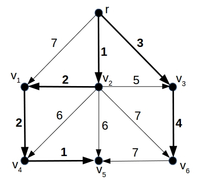

A directed graph <em>G</em> with root node
<em>r</em>
and a cost assigned to each edge

A directed graph G with root node r and a cost assigned to each arrow. The minimum cost arborescence for this graph is indicated in bold. For example, the path {r, v₂, v₁, v₄} from the root node r to node v₄ has a lower cost (1+2+2=5) than the two shorter paths {r, v₁, v₄} (7+2=9) and {r, v₂, v₄} (1+6=7).

Given a directed graph

G

with a root and a cost function, there are algorithms that find you a minimal cost arborescence in a reasonable amount of time (for experts, the problem is in the complexity class P). Such algorithms were proposed independently first in 1965 by Yoeng-Jin Chu and Tseng-Hong Liu (who called it a shortest arborescence), then in 1967 by Jack Edmonds (who called it an optimum branching), and finally in 1971 by F. Bock (who called it a minimum spanning tree in a directed network). These algorithms are all based on well-known and efficient minimum cost spanning tree algorithms for undirected graphs, with a recursive extension to check for, and resolve, potential cycles. Later on, an improvement was made by Robert Tarjan, resulting in an even more efficient algorithm.

Reconstructing dispersal routes

When you are trying to reconstruct the route along which a species, such as the spotted knapweed, has dispersed you usually have the following pieces of information:

A number $n$ of geographic locations where the species has been observed. The locations are points on the map, so we can give them coordinates $(x_{1}, y_{1})$ , $(x_{2}, y_{2})$ , etc, up to $(x_{n}, y_{n})$ .
For each location there is a time at which the particular species of interest was first observed at that location. We write $t_{1}$ for the time corresponding to the location $(x_{1}, y_{1})$ , etc, up to $t_{n}$ for the time corresponding to the location $(x_{n}, y_{n})$ .

Using this information we can construct a directed graph $G$ with a root. Each node in the graph corresponds to one of the locations $(x_{i}, y_{i})$ (where $i$ runs from $1$ up to $n$ ). We connect one node to another by an arrow pointing from the first to the second node if the time associated to the first node is earlier than the time associated to the second node. The root node is the one with the earliest associated time. The cost associated to an arrow is the (Euclidean) distance between the two locations represented by the nodes it connects.

Assuming that a location is always invaded from the nearest earlier occupied location, it doesn't take much thought to see that finding the minimum cost arborescence for the graph $G$ immediately provides the most likely dispersal routes of the given species. The figure below shows the most likely dispersal routes for spotted knapweed in North America, based on historical data of first occurrences in many different locations, using the arborescence method as described above.

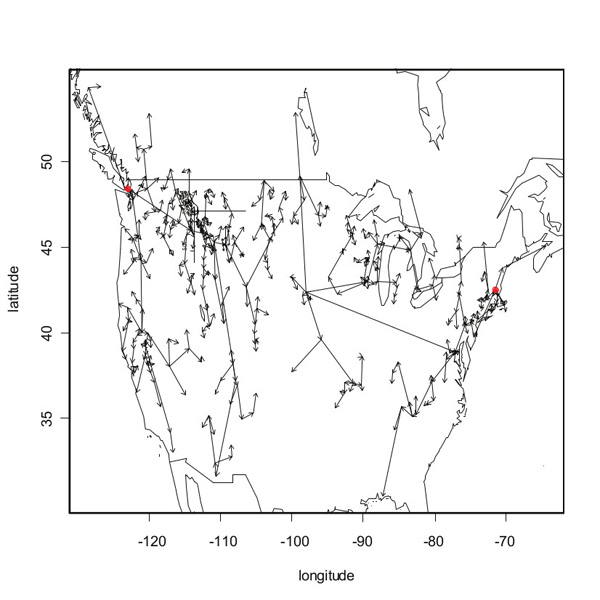
The most likely disperal routes of spotted knapweed in North America

The most likely dispersal routes of spotted knapweed in North America, as reconstructed using the minimum cost arborescence method. The two red dots indicate the two (independent) introduction sites.

My colleague Olivier Broennimann and I published this formal correspondence between the dispersal routes reconstruction problem in ecology and the minimum cost arborescence problem in mathematics in an article in the Journal of Theoretical Biology.

Generalisations and other applications

Some of the assumptions underlying the method above are rather simplistic. For example, an invasion event may not always happen from the nearest already occupied location. There may be a barrier between two locations, such as a river or a mountain, that prevents the dispersal from one location to another. Or dispersal may depend on predominant wind direction (such as with plant seeds), which may preclude dispersal in certain directions. Such cases can be dealt with by setting the cost value of the arrow connecting the two locations to a very large value or even infinity. In other words, the cost function can be easily adjusted according to "real world" situations, to take geographical, climatic, or biological constraints into account.

Cute or not, the common bushtail possum is an invader.

There is also likely to be some noise in the data in terms of the first occurrence times. In the data set, the times $t_{i}$ indicate the first time a given species was observed in a given location. However, this means that the actual time of invasion may have been some time before $t_{i}$ . To take this into account we can, for example, subtract some random value from each $t_{i}$ and run the minimum cost arborescence algorithm on multiple "randomised" instances. This way, a confidence score can be assigned to each arrow in the most likely dispersal routes, by counting in how many of these random instances that same arrow is included in the resulting minimum cost arborescence.

Why do we do it?

Being able to reconstruct the most likely dispersal routes of invasive species has important practical applications. For example, it can help in the design and implementation of quarantine strategies, or of conservation actions such as preventing the establishment of new "seed" populations, rather than focusing on established invasion fronts. Furthermore, the method as described here can be used to study various "what if?" scenarios. Both the data and the cost function can be adjusted to reflect hypothetical (possibly even future) scenarios, for which it can then be studied how that affects the most likely dispersal of invasive species.

In conclusion, the ecological dispersal routes reconstruction problem can be stated in terms of a known mathematical problem, for which there exists an efficient algorithm to find the optimal solution. This provides a mathematically sound and versatile tool to study the dynamics of invasive species, thus turning an ecologist's nightmare into a mathematician's dream.

About the author

Wim Hordijk is an independent scientist currently visiting the Santa Fe Institute in the USA. He has worked on many research and computing projects all over the world, mostly focusing on questions related to evolution and the origin of life. More information about his research can be found on his website.