Making the grade

November 2003

Sometimes, mathematics may seem like a collection of procedures and techniques, rather than the beautiful consistent whole it really is. One such collection of rules tells us how to find the slope, or "gradient", at a specific point on a curve described by a function. This is better known as differentiation, and is one part of calculus.

This article is the first of a pair which aim to help students encountering calculus for the first time. You do not need to know how to differentiate in order to follow, so it could be used as an introduction to the subject. However the second article will assume you have encountered differentiation as such a set of rules.

We start by explaining a little about gradients. In particular, we look at which functions do, and which functions do not, have a well defined gradient. Next we calculate the gradients of the two functions $x^2$ and $\sin (x)$ at every point. The message here is not that we want the answers, which, if you have encountered calculus before, you probably know are $2x$ and $\cos (x)$ respectively, but rather the method, which gives us a taste of limits. The topic of limits belongs to a subject known in mathematics as analysis. This is a central core underpinning much of the machinery of applied maths.

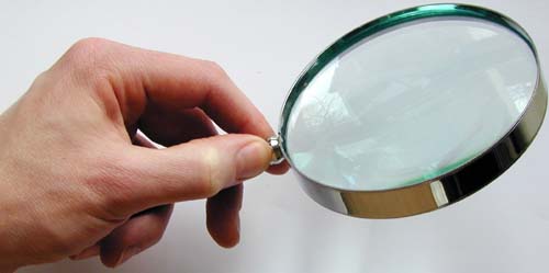
Differentiation: the mathematical magnifying glass.
Image freeimages.co.uk

In the next article we will briefly recap how to avoid the case-by-case arguments we have used here by manipulating the algebraic expressions with which we usually describe functions. This is differentiation as we know and love it! We will also think about how functions are built from component parts, and how we differentiate a function by considering these parts individually and how they are combined.

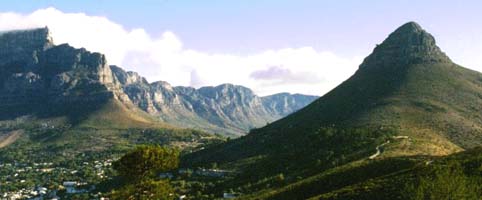
View of Table Mountain, Cape Town, South Africa

Slopes will never look the same again.
Image DHD Photo Gallery

Gradients

Let's start with a simple example, by considering the straight line shown in figure 1 below. The gradient of the line is defined to be

$\begin{equation} \frac{\mbox{Change in } y}{\mbox{Change in }x}. \end{equation}$

(1)

If we take any two distinct points $(x_1,y_1)$ and $(x_2,y_2)$ on the line, the gradient is defined as

$m:=\frac{y_2-y_1}{x_2-x_1},$

which doesn't depend on which points we take. Defining $m$ in this way, the equation of the line is

$y=mx+c,$

where $c$ is the value of $y$ at the point where the line crosses the $y$ -axis.

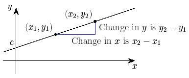
Figure 1: The gradient of a straight line

But what should we do with curves that are not straight, such as the graph of the function $x^2$ , shown in Figure 2 below? Let's choose the point $x=3$ , and try to decide what it means for the curve to have a gradient at the point $(3,9)$ . What we'll do is draw a "tangent line", and find the gradient of this straight line. The gradient of the curve will be defined to be the gradient of this line. We risk a horrible circular argument here because we want to take a straight line which "has the same gradient as the function $x^2$ at that point". But since we haven't a clue what the gradient is yet, we can't! Instead, let's try to make some sense of what a tangent line could be.

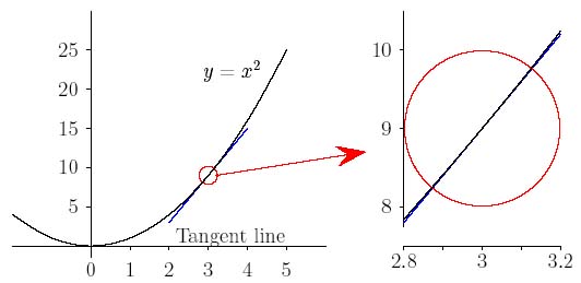
Finding the gradient of y=x<sup>2</sup> at x=3

Figure 2: Finding the gradient of y=x² at x=3

So, imagine you have a magnifying glass or microscope and you take a closer look at the function around the point $(3,9)$ . Imagine you can increase the zoom and keep zooming in to get a closer look at the function around the point (3,9). If you do this, very soon the curve seems to straighten out. For very high magnifications, the curve $x^2$ actually looks like a straight line. We say that at the point $(3,9)$ the function $x^2$ appears to become straight under magnification. So, we attempt to define the gradient of $x^2$ at $x=3$ as the gradient of the straight line which appears under very high magnification.

A note of caution, though. It is very important indeed that you magnify in both the $x$ and $y$ directions equally and simultaneously. If, for example, you continually stretch the $x$ -axis, the function will eventually appear to become flat! This is very misleading.

As you may already know, the formal process of differentiation allows us to calculate the value of this gradient at any point on a function that appears to become straight under magnification, not just at $(3,9),$ say. In a moment we will demonstrate that the gradient of the curve $x^2$ at a point is $2x$ , by examining a limiting argument.

Have a look at the graph below. This looks very complicated but it too appears to become straight under magnification. A small area around $x=0.4246...$ has been magnified twenty times. In fact, if we magnified the function further it would quickly appear to be locally straight, and we could decide how to draw a tangent line.

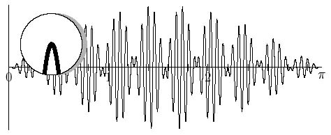
Figure 3: A "spiky" function which is actually smooth, and even appears to become straight under magnification

So just looking casually at the graph itself is not necessarily a good guide as to whether the function appears to become straight under magnification, or not. However many commonly encountered functions, such as polynomials, and also the functions $\sin (x)$ , $\cos (x)$ and $e^ x$ , will appear to become straight under magnification. Simply applying the formal rules of calculus in a mechanical way, without giving much thought to what you are doing, is also fraught with danger. The very fact that calculus is so effective, and the wealth of functions to which calculus may be applied, sometimes lulls the careless into thinking that all functions appear to become straight under magnification.

Some functions which do not become straight under magnification

An example of a function which does not appear to become straight under magnification at the point $x=0$ is $|x|$ , which is defined as

$|x|:= \left\{ \begin{array}{ll} x, & x\geq 0,\\ -x, & x < 0. \end{array} \right.$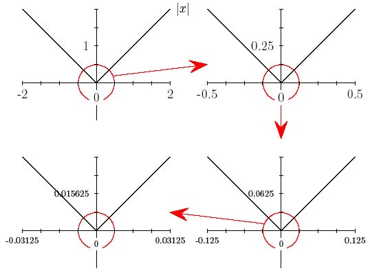

Figure 4: The graph of |x| at various magnifications

The graph of $|x|$ is shown above under different degrees of magnification. It always appears "kinked" around the point $(0,0)$ . We can never fit a straight tangent line to the curve at the point $(0,0)$ . However, away from the point $(0,0)$ , $|x|$ is straight. The gradient of the function away from $0$ is $1$ if $x>0$ and $-1$ when $x<0$ , which is simply the algebraic sign of $x$ , sometimes written as sgn $(x)$ :

$\mbox{sgn}(x):= \left\{ \begin{array}{ll} 1, & x>0,\\ -1, & x < 0,\\ \mbox{undefined}, & x=0. \end{array} \right.$

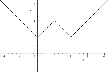
Figure 5: The function f(x) = |x|-|x-1|+|x-2|

There are many other functions which do not become straight under magnification. Simply adding together shifted versions of $|x|$ , such as $|x-1|$ , will allow us to produce many different functions with "kinks". For example, the graph of the function $f(x) = |x|-|x-1|+|x-2|$ is shown to the left.

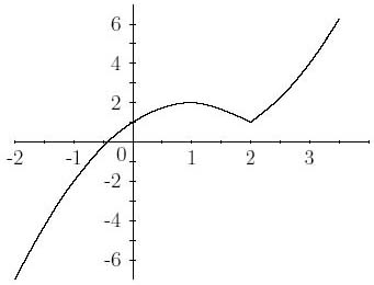
Figure 6: The function f(x)=x|x-2| + 1

And shown to the right is the function $f(x)=x|x-2|+1$ . This has a kink at $x=2$ , but is not made of straight line sections.

In addition, it is possible to produce functions with an infinite number of such bad points. In fact, the graph shown below is of a continuous function which has a "kink" at every point! More correctly, we cannot define the gradient at any point of the curve.

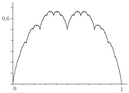
Figure 7: A function which does not become straight under high magnification anywhere

Examples such as this were ignored as monsters by some 19th century mathematicians who argued about whether they were even functions. However, these are what make mathematics surprising and interesting. In fact, such examples are much more common that experience applying calculus to textbook examples would lead us to believe. Importantly, such objects, known as fractals, turn out to be very useful for describing the shapes of physical objects such as mountains, coast lines, fractures, cracks and so on. This is perhaps the most famous example, and is constructed by adding together an infinite number of of saw-tooth-like functions.

Other examples are a little easier to handle algebraically, but it is harder to prove they are "monstrous". Two such examples are

$\begin{equation} f(x) = \sum _{n=1}^\infty \frac{\sin (n^2 x)}{n^2} = \sin (x)+\frac{\sin (4x)}{4} + \frac{\sin (9x)}{9} +... \end{equation}$

(1)

and

$f(x) = \sum _{n=1}^\infty \frac{\sin (n! x)}{n!} = \sin (x)+\frac{\sin (2x)}{2} + \frac{\sin (6x)}{6} +...$

You might like to use a computer to approximate these functions by plotting the first few terms in each series. For the first of these functions you start by plotting

$\sin (x),$

then plot

$\sin (x) + \frac{\sin (4x)}{4},$

then

$\sin (x)+\frac{\sin (4x)}{4} + \frac{\sin (9x)}{9},$

and so on. You will soon see an intricately detailed function evolve.

Calculating gradients of some simple functions

So far, we have done very little mathematical calculation or problem solving, and only discussed what happens when we look at the graphs of curves under magnification. Now we will try to calculate the gradient of a curve by manipulating the formula for the curve itself. We will calculate from first principles the gradient at every point of the two very familiar basic functions: $x^2$ and $\sin (x)$ . Although you may already know the answers - $2x$ and $\cos (x)$ respectively - we are really interested in the method for finding them. Then we explain what goes wrong when we try to apply this method to the function $|x|$ at $x=0$ .

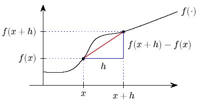
Figure 8: Calculating the gradient of a general function

To the left is the graph of a function $f(x)$ , and the point $x$ at which we want to try to define the gradient. One way to think about the gradient is to draw a straight line connecting the points $(x,\, f(x))$ and $(x+h,\, f(x+h))$ on the curve. We may calculate the gradient of this straight line using equation (1): it is equal to $\frac{\mbox{change in $y$}}{\mbox{change in $x$}}.$ This quantity is the change in $f(x)$ divided by the change in $x$ , and this gradient is

$\frac{f(x+h)-f(x)}{h} \quad \mbox{for all $h\neq 0$.}$

Since we are interested in functions that appear to be straight under very high magnification, we are most interested in what happens when $x$ and $x+h$ are close together. This happens for very small positive and negative $h$ . The gradient of the line in the diagram above will then be very close to the gradient of the function, which now appears straight. Note that the diagram only shows the situation for $h>0$ and also when $h$ is quite large. You will have to imagine for yourself what happens when $h$ is small, or when $h<0$ . Here we can’t set $h=0$ as that would mean dividing by zero, which makes no sense.

The function x²

Let us consider the concrete example $f(x)=x^2$ . Calculating the formula

$\begin{equation} \frac{f(x+h)-f(x)}{h} \quad \mbox{ for all } h\neq 0 \end{equation}$

(2)

gives

$\frac{f(x+h)-f(x)}{h} = \frac{(x+h)^2-x^2}{h} = \frac{x^2+2xh+h^2-x^2}{h} =2x+h.$

If $h$ is very small - positive or negative - we may approximate $2x+h$ as $2x$ . If we think about what happens as $h$ gets very small indeed, in the limit we have the slope of the tangent line. By a limiting argument, which can be made watertight mathematically, we say that the function $f(x)=x^2$ does indeed become straight under magnification because we can make sense of the slope of the chord, in the limit when $h$ is very small indeed. The limiting slope of the chord defines the slope of the tangent. In this case the limit is $2x$ . Therefore, we say the gradient of the tangent line is $2x$ , although in this case we knew that already.

The function sin(x)

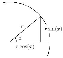
Figure 9: The definition of the trigonometrical functions sin(x) and cos(x)

Next we attempt to deal with the function $\sin (x)$ . Recall that if $x$ is an angle in a right angle triangle with hypotenuse $r$ , $\sin (x)$ is the length of the opposite side, as shown to the left, which in our case is the length of the vertical side of the triangle.

Before we calculate the gradient of $\sin (x)$ we need to think for a moment about angles, and more particularly about the units with which we measure angles. Recall that given a circle of radius $r$ , the circumference is $2\pi r$ . If we have a fraction $x$ of a whole circle we have arc length $2\pi rx$ . Generally we don't talk about fractions of a circle, but rather an angle measured with some system of units. Two common methods are to use $360$ degrees, or $2\pi$ radians. If we use an angle $h$ , the arc length will be $krh$ , where $k$ is a constant that depends on the units of angle you use. If we use radians, then $k=1$ , which is the whole point of using radians! Therefore, if we have an angle $h$ measured in radians, the arc length is simply $rh$ .

To calculate the gradient on the curve of $\sin (x)$ , we need to evaluate

$\frac{\sin (x+h)-\sin (x)}{h}.$

To do this we examine the diagram below, which gives us a clue as to how to estimate $\sin (x+h)$ .

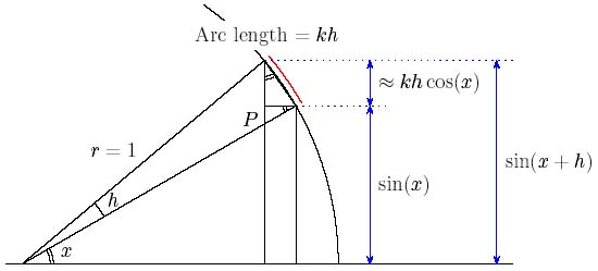
Figure 10: Calculating sin(x+h)

Here we have taken r=1. Each occurrence of the angle x is marked with a . Next we approximate the hypotenuse of the small triangle with right angle at $P$ , as the arc length of the circle, which is $kh$ . For small values of $h$ , which we need to consider when finding the gradient, this is a very good approximation indeed. Therefore, since we have taken the radius $r=1$ , we have

$\sin (x+h) = \sin (x) + kh\cos (h),$

and so

$\frac{\sin (x+h)-\sin (x)}{h} = \frac{\sin (x) + kh\cos (h)-\sin (x)}{h} = k\cos (x).$

Therefore the gradient of $\sin (x)$ is equal to $k\cos (x)$ . Recall, the constant $k$ depends on the units we use to measure the angle. If we use radians then $k=1$ . This is the reason for adopting radians in mathematics, rather then degrees which are very convenient for more practical measuring purposes. Although $h$ does not appear in this formula, we assumed that $h$ was small in order to estimate the hypotenuse as the arc length. This allows us to calculate the gradient of the curve $\sin (x)$ at the point $x$ .

The function |x|

The diagrams in Figure 4 show convincingly that $|x|$ is not locally straight at $x=0$ . What happens if we try to calculate the quantity in formula (2) in this case? Well,

$\frac{f(0+h)-f(0)}{h} = \frac{|h|}{h}.$

If $h>0$ , then $|h|=h$ and so this quantity equals $1$ . On the other hand, for all $h<0$ , $|h|=-h$ , so this quantity equals $-1$ . Thus as we approach $0$ from the positive direction the gradient appears to be $1$ , and from the negative direction the gradient appears to be $-1$ . Since these do not agree, we cannot define the gradient at $0$ in a meaningful way. This confirms that $|x|$ is indeed not straight under magnification at $x=0$ .

In the next article we will continue this discussion and examine some formal rules which drastically reduce the effort necessary to calculate the gradient. We will also think about about how functions are built up in different ways, and how these rules are applied in much more complex situations.

Exercises

The following exercises are suggestions of things you could work on to test whether you can adapt the arguments above to a new situation. There are no answers here to encourage you to work on them yourself.

Redraw Figure 8 showing the situation when $h<0$ and small.
Sketch on the same axes and compare
- $|x|$ and its derivative sgn $(x)$ ,
- $x^2$ and its derivative $2x$ ,
- $x^3$ and its derivative $3x^2$ ,
Apply formula (2) to the following functions and simplify them as far as possible. Try to write your answer in the form , where depends only on , not on .
- $f(x)=x^3$ ,
- $f(x)=x^4$ ,
- $f(x)=2x^2+x^3$ .
What happens when becomes very small? What can you say about ?
Apply formula (2) to the function

$f(x)=\frac{1}{x}.$

Write your answer as a single fraction. What happens when $h$ becomes very small?
Adapt the diagram in Figure 10 and try to work through the argument given to show that

$\frac{d}{dx} \cos (x) = -\sin (x).$

Instead of approximating $\sin (h)\approx h$ for very small $h$ , you might need to use $\cos (h)\approx 1-\frac{h^2}{2}$ for very small $h$ .
Give an example of
- a function with a "kink" at $x=2$ .
- a function with "kinks" at $x=1$ , $x=2$ , and $x=3$ .

Sketch, using a computer, the functions

$\displaystyle f_1(x)$	$\displaystyle =$	$\displaystyle \sin (x),$
$\displaystyle f_2(x)$	$\displaystyle =$	$\displaystyle \sin (x) + \frac{\sin (4x)}{4},$
$\displaystyle f_3(x)$	$\displaystyle =$	$\displaystyle \sin (x)+\frac{\sin (4x)}{4} + \frac{\sin (9x)}{9}.$

If possible, sketch

$f_ n(x)=\sin (x)+\frac{\sin (4x)}{4} + \cdots + \frac{\sin (n^2x)}{n^2}$

for larger $n$ . Try, in your mind's eye, to relate these partial sums to the infinite sum

$f_\infty (x) = \sum _{n=1}^\infty \frac{\sin (n^2 x)}{n^2} = \sin (x)+\frac{\sin (4x)}{4} + \frac{\sin (9x)}{9} + \cdots$

About the author

Chris Sangwin is a member of staff in the School of Mathematics and Statistics at the University of Birmingham. He is a Research Fellow in the Learning and Teaching Support Network centre for Mathematics, Statistics, and Operational Research. His interests lie in mathematical Control Theory.

Chris would like to thank Mr Martin Brown, of Thomas Telford School, for his helpful advice and encouragement during the writing of this article.

Comments

graph

the graph of y=|x|-|x-1|+|x+2| is not like Figure 5.
If we choose x= 0 the value of y is 1. But in figure 5, for x = 0 value of y is 0.

Thans for pointing that out!

Thans for pointing that out! We have replaced the picture with a correct one.