Chaos in Numberland: The secret life of continued fractions
Different ways of looking at numbers
There are all sorts of ways of writing numbers. We can use arithmetics with different bases, fractions, decimals, logarithms, powers, or simply words. Each is more convenient for one purpose or another and each will be familiar to anyone who has done some mathematics at school. But, surprisingly, one of the most striking and powerful representations of numbers is completely ignored in the mathematics that is taught in schools and it rarely makes an appearance in university courses, unless you take a special option in number theory. Yet continued fractions are one of the most revealing representations of numbers. Numbers whose decimal expansions look unremarkable and featureless are revealed to have extraordinary symmetries and patterns embedded deep within them when unfolded into a continued fraction. Continued fractions also provide us with a way of constructing rational approximations to irrational numbers and discovering the most irrational numbers.
Every number has a continued fraction expansion but if we restrict our ambition only a little, to the continued fraction expansions of "almost every" number, then we shall find ourselves face to face with a simple chaotic process that nonetheless possesses unexpected statistical patterns. Modern mathematical manipulation programs like Mathematica have continued fraction expansions as built in operations and provide a simple tool for exploring the remarkable properties of these master keys to the secret life of numbers.
The Nicest Way of Looking at Numbers
Introducing continued fractions
Consider the quadratic equation \setcounter{equation}{0} \begin{equation} \htmlimage{} x^2-bx-1=0 \label{A} \end{equation} Dividing by $x$ we can rewrite it as \setcounter{equation}{1} \begin{equation} x=b+\frac 1x \end{equation} Now substitute the expression for $x$ given by the right-hand side of this equation for $x$ in the denominator on the right-hand side: \setcounter{equation}{2} \begin{equation} x=b+\leftb \frac 1{b+\frac 1x} \rightb \end{equation} We can continue this incestuous procedure indefinitely, to produce a never-ending staircase of fractions that is a type-setter's nightmare: \setcounter{equation}{3} \begin{equation} x=b+\leftb \frac 1{b +\frac 1{b+\frac 1{b+\frac 1{b+\ldots}}}} \rightb \label{B} \end{equation} This staircase is an example of a \textit{continued fraction}. If we return to equation 1 then we can simply solve the quadratic equation to find the positive solution for $x$ that is given by the continued fraction expansion of equation 4; it is \setcounter{equation}{4} \begin{equation} x=\frac{b+\sqrt{b^2+4}}2 \label{Ba} \end{equation} Picking $b=1$, we have generated the continued fraction expansion of the \textit{golden mean},$\Phi$: \setcounter{equation}{5} \begin{equation} \Phi =\frac{\sqrt{5}+1}2=1+\frac 1{1+\frac 1{1+\frac 1{1+\frac 1{1+\ldots}}}} \label{B1} \end{equation} This form inspires us to define a general continued fraction of a number as \setcounter{equation}{6} \begin{equation} a_0+\frac 1{ a_1+\frac 1{a_2+\frac 1{a_3+\frac 1{1+\ldots + \frac 1{a_n} + \ldots}}} } \label{C} \end{equation} where the $a_n$ are $n+1$ positive integers, called the \textit{partial quotients} of the continued fraction expansion (cfe). To avoid the cumbersome notation we write an expansion of the form equation 7 as \setcounter{equation}{7} \begin{equation} [ a_0;a_1,a_2,a_{3},\ldots, a_n,\ldots] \label{Ca} \end{equation}
Continued fractions first appeared in the works of the Indian mathematician Aryabhata in the 6th century. He used them to solve linear equations. They re-emerged in Europe in the 15th and 16th centuries and Fibonacci attempted to define them in a general way. The term "continued fraction" first appeared in 1653 in an edition of the book Arithmetica Infinitorum by the Oxford mathematician, John Wallis. Their properties were also much studied by one of Wallis's English contemporaries, William Brouncker, who along with Wallis, was one of the founders of the Royal Society. At about the same time, the famous Dutch mathematical physicist, Christiaan Huygens made practical use of continued fractions in building scientific instruments. Later, in the eighteenth and early nineteenth centuries, Gauss and Euler explored many of their deep properties.
How long is a continued fraction?
Continued fractions can be finite in length or infinite, as in our example above. Finite cfes are unique so long as we do not allow a quotient of $1$ in the final entry in the bracket (equation 8), so for example, we should write 1/2 as $[0;2]$ rather than as $[0;1,1].$ We can always eliminate a $1$ from the last entry by adding to the previous entry. \par If cfes are finite in length then they can be evaluated level by level (starting at the bottom) and will reduce always to a rational fraction; for example, the cfe $[1,3,2,4]=40/31$. However, cfes can be infinite in length, as in equation 6 above. Infinite cfes produce representations of irrational numbers. If we make some different choices for the constant $b$ in equations 4 and 5 then we can generate some other interesting expansions for numbers which are solutions of the quadratic equation. In fact, all roots of quadratic equations with integer coefficients, like equation 5, have cfes which are eventually periodic, like $[2,2,2,3,2,3,2,\ldots]$ or $[2,1,1,4,4,1,1,4,1,1,4,\ldots]$. Here are the leading terms from a few notable examples of infinite cfes: \setcounter{equation}{8} \begin{equation} e=[2;1,2,1,1,4,1,1,6,1,1,8,1,1,10,\ldots] \label{C1} \end{equation} \setcounter{equation}{9} \begin{equation} \sqrt{2}=[1;2,2,2,2,2,2,2,2,2,2,2,2,2,2,2,\ldots] \label{C2} \end{equation} \setcounter{equation}{10} \begin{equation} \sqrt{3}=[1;1,2,1,2,1,2,1,2,1,2,1,2,1,2,\ldots] \label{C3} \end{equation} \setcounter{equation}{11} \begin{equation} \pi =[3;7,15,1,292,1,1,1,2,1,3,1,14,2,1,1,2,2,2,2,1,84,2,\ldots] \label{C4} \end{equation} These examples reveal a number of possibilities. All of the expansions except that for $\pi$ have simple patterns whilst that for $\pi$, which was first calculated by John Wallis in 1685, has no obvious pattern at all. There also seems to be a preference for the quotients to be small numbers in these examples. The cfe for $e$ was first calculated by Roger Cotes, the Plumian Professor of Experimental Philosophy at Cambridge, in 1714.Continued fractions allow us to probe an otherwise hidden order within the realm of numbers. If we had written the number $\Phi$ as a decimal ($1.61803\ldots$) or even in binary ($1.100111\ldots$) then it looks a pretty nondescript number. Only when it is written as a continued fraction does its unique structure emerge.
Some Useful Applications
Approximating Pi
If we chop off an infinite cfe after a finite number of steps then we will create a \textit{rational approximation} to the original irrational. For example, in the case of $\pi$, if we chop off the cfe at $[3;7]$ we get the familiar rational approximation for $\pi$ of $22/7=3.1428571\ldots$. If we keep two more terms then we have $[3;7,15,1]=355/113=3.1415929\ldots$, an even better approximation to $\pi =3.14159265\ldots$.This approximation was known to the early Chinese. The first eight rational approximations are \setcounter{equation}{12} \begin{equation} \frac 31,\frac{22}7,\frac{333}{106},\frac{355}{113},\frac{103993}{33102}, \frac{104348}{33215},\frac{208341}{66317},\frac{312689}{99532} \end{equation} The more terms we retain in the cfe, the better the rational approximation becomes. In fact, the cfe provides the best possible rational approximations to a general irrational number. Notice also that if a large number occurs in the expansion of quotients, then truncating the cfe before that will produce an exceptionally good rational approximation. Later on we shall see that, in some sense, it is probable that most cfe quotients are small numbers ($1$ or $2$), so the appearance in the cfe of $\pi$ of a number as large as $292$ so early in the expansion is rather unusual. It also leads to an extremely good rational approximation to $\pi =[3;7,15,1,292]=103993/33102.$Pythagorean musical scales
The ancient Pythagoreans discovered that the division of the string of a musical instrument by a ratio determined by small integers resulted in an appealing relationship. For example, a half length gives a frequency ratio of $2:1$, the musical octave, and a third length gives a ratio of $3:2$, the musical fifth, a quarter length gives a frequency ratio $4:3$, the musical fourth, a frequency ratio $5:4$, the major third. We can now ask how the Pythagorean scale fits together. For example, how many major thirds equal an integral number of octaves; that is, when is \setcounter{equation}{13} \begin{equation} \left( \frac 54\right) ^b=2^a ? \end{equation} Taking logarithms to the base $2$, we are looking for a solution $\log_25=2+a/b$. Since the $\log$ is irrational there cannot be any exact solutions for integers $a$ and $b$. But there are "almost" solutions. To find them we just look at the cfe of $\log _25=2.3219\ldots=[2;3,9,\ldots]$. Chopping it after the first fractional term gives the rational approximation $\log _25\approx 2+\frac 13$, so the approximate solution to our problem is $a=1$, $b=3$, and \setcounter{equation}{14} \begin{equation} \left( \frac 54\right) ^3=1.95\ldots\approx 2 \end{equation} If we used the next cf approximant we would get $a=9,b=28$ which is rather awkward to handle.Gears without tears
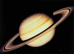
Saturn
Huygens was building a mechanical model of the solar system and wanted to
design the gear ratios to produce a proper scaled version of the planetary
orbits. So, for example, in Huygens' day it was thought that the time
required for the planet Saturn to orbit the Sun is $29.46$ years (it is now
known to be $29.43$ years). In order to model this motion correctly to
scale, he needed to make two gears, one with $P$ teeth, the other
with
$Q$ teeth, so that $P/Q$ is approximately $29.46$. Since it is hard to fashion
small gears with a huge number of teeth, Huygens looked for relatively small
values of $P$ and $Q$. He calculated the cfe of $29.46$ and read off the
first few rational approximations: $\frac{29}1,\frac{59}2,\frac{206}7$.
Thus, to simulate accurately Saturn's motion with respect to that of the
Earth's, Huygens made one gear with $7$ teeth and the other with $206$
teeth.
A schematic of Huygens' gear train
One of Ramanujan's tricks revealed
The remarkable Indian mathematician Srinivasa Ramanujan (1887-1920) was famous for his uncanny intuition about numbers and their inter-relationships. Like mathematicians of past centuries he was fond of striking formulae and would delight in revealing (apparently from nowhere) extraordinarily accurate approximations (can you show that $2^{10}\approx 10^3$ ?). Ramanujan was especially fond of cfes and had an intimate knowledge of their properties. Knowing this one can see how he arrived at some of his unusual approximation formulae. He knew that when some irrational number produced a very large quotient in the first few term of its cfe then it could be rationalised to produce an extremely accurate approximation to some irrational. A nice example is provided by Ramanujan's approximation to the value of $\pi$, \setcounter{equation}{15} \begin{equation} \pi \approx \left( \frac{2143}{22}\right) ^{\frac 14} \end{equation} which is good to $3$ parts in $10^4$. How did he arrive at this? Knowing of his fascination with continued fractions we can guess that he knew something interesting about the cfe of $\pi^4$. Indeed, there is something interesting to know: quotient number six in the continued fraction expansion of $\pi ^4$ is huge: \setcounter{equation}{16} \begin{equation} \pi ^4=[97;2,2,3,1,16539,1,\ldots] \label{D4} \end{equation} By using the rational approximation that comes from truncating the cfe before $16539$ you get a remarkably accurate approximation to $\pi ^4$; now just take its fourth root. Ramanujan was also interested in other varieties of nested expansion. In 1911 he asked in an article in the \textit{Journal of the Indian Mathematical Society} what the value was of the following strange formula, an infinite nested continued root: \setcounter{equation}{17} \begin{equation} ?=\sqrt{1+2\sqrt{1+3\sqrt{1+\ldots}}} \end{equation} A few months went by and no one could supply an answer. Ramanujan revealed that the answer is simply $3$ and proved a beautiful general formula for continued roots: \setcounter{equation}{18} \begin{equation} x+1=\sqrt{1+x\sqrt{1+(x+1)\sqrt{1+\ldots}}} \end{equation} Applied mathematicians have found that by approximating functions by continued function expansions, called Pad\'e approximants, they often obtain far more accurate low-order approximations than by using Taylor series expansions. By truncating them at some finite order, they end up with an approximation that is represented by the ratio of two polynomials.Rational approximations - how good can they get?
Minding your p's and q's
Continued fractions allow us to probe an otherwise hidden order within the realm of numbers. If we had written the decimal part of the number $\Phi$ ($0.61803\ldots$) or even in binary ($0.100111\ldots$) then it looks a pretty nondescript number. Only when it is written as a continued fraction does its unique status emerge. The rational fractions which are obtained by chopping off a cfe at order $n$ are called the \textit{convergents} of the cf. We denote them by $p_n / q_n$. As $n$ increases, the difference between an irrational $x$ and its convergent decreases \setcounter{equation}{19} \begin{equation} \left| x-\frac{p_n}{q_n}\right| \rightarrow 0 \end{equation} how quickly? \par The cfe also allows us to gauge the simplicity of an irrational number, according to how easily it is approximatable by a rational fraction. The number $\Phi-1=(\sqrt{5}-1)/2$ is in this sense the "most irrational" of numbers, converging slowest of all to a rational fraction because all the $a_i$ are equal to $1$, the smallest possible value. In fact, Lagrange showed that for any irrational number $x$ there are an infinite number of rational approximations, $p/q$, satisfying \setcounter{equation}{20} \begin{equation} \left| x-\frac pq\right| \frac 1{q^2\sqrt{5}}, \label{D1} \end{equation} where the statement becomes false if $\sqrt{5}$ is replaced by a larger number. In the case of the rational approximations to $(\sqrt{5}-1)/2$ provided by the cfe, they are $p_n/q_n=0/1,1/1,1/2,2/3,3/5,5/8,\ldots$ as $n\rightarrow \infty$ and they have the weakest convergent rate allowed by equation 21 with \setcounter{equation}{21} \begin{equation} \ \left| x-\frac{p_n}{q_n}\right| \rightarrow \frac 1{q^2\sqrt{5}} as\;n\rightarrow \infty \label{D2} \end{equation} Thus the cfe shows that the golden mean stays farther away from the rational numbers than any other irrational number. Moreover, for any $k\geq 2$, the denominator to the rational approximation produced by truncating the cfe of any number satisfies \setcounter{equation}{22} \begin{equation} q_k\geq 2^{(k-1)/2} \label{D2a} \end{equation} If the cfe is finite then $k$ will only extend up to the end of the expansion. In fact, it is possible to pin down the accuracy of the rational approximation in terms of the denominators, $q_i$, from both directions by \setcounter{equation}{23} \begin{equation} \frac 1{q_k(q_{k+1}+q_k)}\left| x-\frac{p_n}{q_n}\right| \frac 1{q_kq_{k+1}} \label{D3} \end{equation} There are many other interesting properties of cfes but one might have thought that there could not be any very strong properties or patterns in the cfes of all numbers because they can behave in any way that you wish. Pick any finite or infinite list of integers that you like and they will form the quotients $a_n$ of one and only one number. Conversely, any real number you care to choose will have a unique cfe into a finite or an infinite list of integers which form the quotients of its cfe. A search for general properties thus seems hopeless. Pick a list (finite or infinite) of integers with any series of properties that you care to name and it will form the cfe of some number. However, while this is true, if we restrict our search to the properties of the cfes of \textit{almost any} (a.e.) real number -- so omitting a set of 'special numbers' which have a zero probability of being chosen at random from all the real numbers - then there are remarkable \textit{general} properties shared by all their cfes.The Patterns Behind Almost Every Number
Gauss's other probability distribution
The general pattern of cfes was first discovered in 1812 by the great German mathematician Carl Friedrich Gauss (1777-1855), but (typically) he didn't publish his findings. Instead, he merely wrote to Pierre Laplace in Paris telling him what he had found, that for typical continued fraction expansions, the probability $P([0;a_1,a_2,\ldots,a_n,\ldots]Lévy's constant
Paul L\'evy showed that when we confine attention to almost every continued fraction expansion then we can say something equally surprising and general about the rational convergents. We have already seen in equations 21-24 that the rational approximations to real numbers improve as some constant times $q_n^{-2}$ as $n$ increases. It can be shown that, for a.e. number, its $q_n$ cannot grow exponentially fast as $n$ increases ($q_nKhinchin's constant
Then the Russian mathematician Aleksandr Khinchin (1894-1959) proved the third striking result about the quotients of almost any cfe. Although the arithmetic mean, or average, of the $k_i$ does \textit{not} have a finite value, the geometric mean does. Indeed, it has a finite value that is universal for the cfes of almost all real numbers. He showed that as $n\rightarrow \infty$ \setcounter{equation}{27} \begin{equation} (k_1k_2k_3{\ldots}k_n)^{1/n}\rightarrow \kappa \end{equation} where Khinchin's constant, $\kappa$, is given by a slowly converging infinite product \setcounter{equation}{28} \begin{equation} \kappa =\prod\limits_{k=1}^\infty \left\{ 1+\frac 1{k(k+2)}\right\} ^{\frac{\ln k}{\ln 2}}=2.68545\ldots \end{equation} Thus the geometric mean quotient value is about $2.68$, reflecting the domination by small values that we have seen in the probability distribution. Again, it is interesting to see how closely this value is approached by the quotients of $\pi$. \par If we list the appearance of different values of $k=1,2,3,\ldots$ etc amongst the first $100$ terms in the cfe of $\pi$, then the $k$ values and their frequencies $N(k)$ in decreasing order of appearance, are as follows: \begin{tabular}{cccccccccccccccccccccc} $k$ & $1$ & $2$ & $3$ & $4$ & $5$ & $6$ & $7$ & $8$ & $15$ & $10$ & $12$ & $13$ & $14$ & $16$ & $22$ & $24$ & $45$ & $84$ & $99$ & $161$ & $292$ \\ $N(k)$ & $41$ & $22$ & $7$ & $4$ & $2$ & $5$ & $3$ & $2$ & $2$ & $1$ & $1$ & $1$ & $1$ & $1$ & $1$ & $1$ & $1$ & $1$ & $1$ & $1$ & $1$ \end{tabular} We see that there is already quite good convergence to the predicted values of $P(k)$ for the small values of $k$. If we calculate the geometric mean, then we find even better convergence to Khinchin's constant, \setcounter{equation}{29} \begin{equation} \left( k_1k_2k_3{\ldots}k_{100}\right) ^{\frac 1{100}}=2.6831468 \end{equation} Remarkably, if you calculate the cfe of Khinchin's constant itself you will find that its terms also have a geometric mean that approaches Khinchin's constant as their number approaches infinity.A notable exception
The most important number that is not a member of the club of "almost every number" whose geometric mean $k$ value approaches Khinchin's is $e=2.71828\ldots$. From equation 9, it is easy to work out what happens to the geometric mean as $n\rightarrow \infty$. All the $1$'s do nothing to the product of the $k$'s and what remains is just twice the product of successive numbers, which introduces $n!$ and so we can use a good approximation for it, like Stirling's, to show that as $n\rightarrow \infty$ \setcounter{equation}{30} \begin{equation} (k_1(e)k_2(e){\ldots}k_n(e))^{\frac 1n}\rightarrow \left( \frac{2n}{3e} \right) ^{\frac 13}=0.62595n^{\frac 13}. \end{equation}Chaotic Numbers
Numbers as chaotic processes
The operation of generating the infinite list of cfe quotients from a.e. real number is a chaotic process. Suppose the real number we wish to expand is $u_1$ and we split it into the sum of its integer part (denoted $k$) and its fractional part (denoted $x$), so \setcounter{equation}{31} \begin{equation} \htmlimage{} u_1=k+x_1 \end{equation} Sometimes we write $k=[u]$ to denote taking the integer part; for example $[\pi ]=3,[e]=2$. Now if we start with a number like $\pi$, the first quotient $k_{1}$ is just $[\pi ]=3$, and the fractional part is $x_1=0.141592$. The next quotient is the integer part of the fractional part, $k_2=[1/x_1]=[1/0.141592\ldots]=[7.0625459\ldots]=7$; the next fractional part is $x_2=0.0625459\ldots$, and so $k_3=[1/x_2]=[1/0.0625459\ldots]=[15.988488\ldots]=15$. This simple procedure gives the first few quotients of $\pi$, that we listed above in equation 12. The fractional parts (by definition) are always real numbers between $0$ and $1$. They cannot be equal to $0$ or $1$ or the number $u$ would be a rational fraction and the cfe would be finite. The process of generating successive fractional parts is given by a non-linear difference equation which maps $x$ into $1/x$ and then subtracts the integer part: \setcounter{equation}{32} \begin{equation} x_{n+1}=T(x_n)=\frac 1{x_n}-\left[ \frac 1{x_n}\right] \label{Gau} \end{equation} The function $T(x)$ is composed of an infinite number of hyperbolic branches.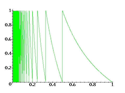
Graph 1: The function T(x) (equation 33).
If we apply this mapping over and over again from almost any starting value
given by a real number with an infinite cfe, then the output of values of $x$
approaches a particular probability distribution, first found by Gauss:
\setcounter{equation}{33}
\begin{equation}
p(x)=\frac 1{(1+x)\ln 2} \label{E}
\end{equation}
Again, as with any probability distribution, we can check that
$\int\limits_0^1p(x)dx=1$.
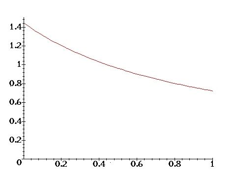
Graph 2: The probability distribution p(x) (equation 34).
What is chaos?
In order for a mapping like $T$ to be chaotic it must amplify small differences in values of $x$ when the mapping is applied over and over again. This requires the magnitude of its derivative $\left| dT/dx\right|$ to be everywhere greater than $1$. Since $dT/dx=-1/x^2$ and $0Continued Fractions in the Universe
Continued fractions appear in the study of many chaotic systems. If a problem of dynamics reduces to the motion of a point bouncing off the walls of a non-circular enclosure, of which the game of billiards is a classic example, then continued fraction expansions of the numbers fixing the initial conditions will describe many aspects of the dynamics as a sequence of collisions occurs. A striking example of this sort has been discovered in the study of solutions in the general theory of relativity, which describe the behaviour of possible universes as we follow them back to the start of their expansion, or follow the behaviour of matter as it plummets into the central singularity of a black hole. In each of these cases, a chaotic sequence of tidal oscillations occurs, whose statistics are exactly described by the continued fraction expansion of numbers that specify their starting conditions. Even though the individual trajectory of a particle falling into the black hole singularity is chaotically unpredictable, it possesses statistical regularities that are determined by the general properties of cfes. The constants of Khinchin and L\'evy turn out to characterise the behaviour of these problems of cosmology and black hole physics.
The Solar System
Continued fractions are also prominent in other chaotic orbit problems. Numbers whose cfes end in an infinite string of $1$s, like the golden mean, are called \textit{noble} numbers. The golden mean is the "noblest" of all because all of its quotients are $1$s. As we have said earlier, this reflects the fact that it is most poorly approximated by a rational number. Consequently, these numbers characterise the frequencies of undulating motions which are least susceptible to being perturbed into chaotic instability. Typically, a system which can oscillate in two ways, like a star that is orbiting around a galaxy and also wobbling up and down through the plane of the galaxy, will have two frequencies determining those different oscillations. If the ratio of those frequencies is a rational fraction then the motion will ultimately be periodic, but if it is an irrational number then the motion will be non-periodic, exploring all the possibilities compatible with the conservation of its energy and angular momentum. If we perturb a system that has a rational frequency ratio, then it can easily be shifted into a chaotic situation with irrational frequencies. The golden ratio is the most stable because it is farthest away from one of these irrational ratios. In fact, the stability of our solar system over long periods of time is contingent upon certain frequency ratios lying very close to noble numbers. \par Continued fractions are a forgotten part of our mathematical education but their properties are vital guides to approximation and important probes of the complexities of dynamical chaos. They appear in a huge variety of physical problems. I hope that this article has given a taste of their unexpected properties.
Further Reading:
-
J.D. Barrow, "Chaotic Behaviour in General Relativity", Physics Reports 85, 1 (1982).
-
G.H. Hardy and E.M. Wright, An Introduction to the Theory of Numbers, Oxford University Presss, 4th ed. (1968).
-
A.Y. Khinchin, Continued Fractions, University of Chicago Press (1961).
-
C.D. Olds, Continued Fractions, Random House, NY (1963).
-
M. Schroeder, Number Theory in Science and Communication, 2nd edn., Springer (1986).
-
D. Shanks and J.W. Wrench, "Khinchin's Constant", American Mathematics Monthly 66, 276 (1959)
-
J.J. Tattersall, Elementary Number Theory in Nine Chapters, Cambridge University Press (1999).
About the author

John D. Barrow is a Professor in the Department of Applied Mathematics and Theoretical Physics at the University of Cambridge.
He is the Director of our own Millennium Mathematics Project.
Comments
Anonymous
When I worked the Saturn problem, I found the 29/1, 59/2, 206/7 ... sequence results from assuming the period is 29.43 years, not from 29.46. Do you have those reversed?
Respectfully,
Crawford Sachs
CLSachs@compuserve.com
Anonymous
Thanks Professor, for the lucid presentation....How CFE's are related to Mendelbrot set?
Srinivasan Nenmeli
Anonymous
As far as I know the mentioned set is called Mandelbrot set and not Mendelbrot set.
Anonymous
Could you add some books in Chaos Theory in your "further reading"?
Thank you in advance.
Peter Faderbauer
The value of the integral for h in equation 36 is wrong. In the denominator on the right side the natural logarithm of two should not be squared. The correct value of the denominator is
6 ln 2 = ln 64. Therefore h = 2,3731382208312509056434459518945..., but from the right side of equation 36 follows h = 3,423714742537303397493525677565... and that is wrong!
Marianne
Thanks for spotting that, we've corrected it.
ghadeer
Please, can somebody help me to cite this paper... I am writing my thesis paper and I need this paper as a reference, so how can I write its form?. Thanks in advance.
Neil Brown
An excellent, informative, and truly readable article. Thank you very much Professor Barrow.
Just after formula 24, the 2nd occurence of "any" in the following sentence should be "and". Underscores added for contrast.
"Pick any finite or infinite list of integers that you like _any_ they will form the quotients a(n) of one and only one number."
Kiyoshi Utsunomiya
I found this article and read with satisfaction after I searched to confirm and streangthen my ideas.
But, I have to point out two errors that I suppose.
[1] In Page 7, regarding the equation P(k)=ln{1+1/k(k+2) }/ln2 (25),
you mentioned in the last sentence "If we make k large enough to expand the 'binominal theorem' (so that k(k+2) behaves as k^2), then P(k) ~ k^(-2) as k→∞". Its formula is not correct . What I thought at thought is the Taylor Expansion, but I found that it's actually possible when making two differece eauations and summing up those before taking its limit to the infinity:
① 2{ln(k+1)-ln k} - {ln(k+2)-ln k}. ② Then, we have Σ(k=1 to ∞) P(k)=ln2/ln2=1.
I was abe to find with your indication that this process is helpful to understand the Khnchin's Constant in his book "Continued Fractions".
[2] In Page 9, In the example for "A notable exeption", you have written the value as follows:
(k_1(e)k_2(e)...k_n(e))^(1/n) → ( 2n/3e)^(1/3)=0.62595n^(1/3). (31)
But, since e=[2; 1,2,1, 1,4,1, 1,6,1, ・・・, 1,2n,1, ・・・], the total products among the first 3n units is still 2^n*n!, then we have the following relation with the help of Stirling formula as (n!)^(1/n)= n/e+O(lon n) and then,
(k_1(e)k_2(e)...k_3n(e))^(1/3n) → ( 2n/e)^(1/3)=0.90277n^(1/3). (31)#
It has to delete the '3' in the denominator of the lefthand side of (31).