Graphical Methods II: The return of the slime
The story so far ...
It is freezing cold. Snow falls from leaden skies and settles on a thick crust of salt, white on white. A howling gale picks up flakes of snow and crystals of salt and throws them mercilessly at the few remaining intact structures. Inside, slugs huddle together for warmth and comfort from the howling knowledge that they did this to themselves.
It is 50 million years from now and, as you may remember from Graphical Methods I, the world until now was dominated by slugs that had split into two rivalling super powers: Slug State A (SSA) and Slug State B (SSB). Competing for land and food, SSA and SSB had their deadly salty missiles trained on each other, missiles capable of ending the world as slugs knew it. For a few years, the slugs' fate hung in a dangerous balance and then the unthinkable happened: both SSA and SSB launched their entire arsenal of weapons. A foolish flurry of missiles returned them to a caveslug existence.
But life finds a way. It always finds a way.
Habitable islands

Slug world after the disaster
In Graphical Methods I we recounted how slug scientists used mathematics to get to grips with the problem of weapons proliferation. Sadly, slug politicians rarely made time to listen to the scientists, who themselves were often guilty of not stating their case strongly enough. Now, those slugs that survive face seemingly endless wastelands covered in salt — where will they grow food?
Fortunately, "islands" of land remain salt-free, and those slugs and lower animals which make it to these islands can find limited food. But as different plants and animals converge on the islands over time, how does the species diversity of these islands change? Do larger islands have a more diverse species profile? And do "satellite" islands close to larger islands have greater diversity, because it is easier for organisms to get there? Let's imagine a slug with some time on its appendages, sitting on a beach of one such island, scratching diagrams in the sand. To what extent would our slug friend be able to address the above questions?
Caveslug maths
We consider migration to and extinction from such isolated islands of habitability. We won't try too hard to define these terms carefully because the model we will consider is fairly crude anyway. For example, if a group of blonkyfarks — the slugs' favourite meat — arrives at an island one day, eats some snafflegrass, and then decides to move on, does this constitute a migration and extinction all in one day? What about seasonal migrations? A more detailed model would have to answer these questions, but we will simply state that various species arrive at and eventually become established in an island, and may later die out completely. This is migration to, and extinction from the islands. In this basic model, we will consider only the total number of species present in an island, and call this variable N.
First, we say a few words about the assumptions we, and our slug friend, make in our analysis. Extinction and migration of species will vary from season to season and with weather cycles. To combat this kind of fluctuation, we "zoom out" and suppose that a year is actually quite a short length of time. In this way, the wiggles on the graph caused by the seasonal fluctuations are too small to be seen, and our graphs will look smooth. Being thus able to ignore the influence of seasons and weather, we note that the migration and extinction can also depend on the types of species present. For example, if all of the species eat snafflegrass, then it won't be long before the snafflegrass is gone and all the species die out. In this discussion, however, we will only consider the effect of island size and distance from other islands from which species might migrate.
By the migration or extinction rate we mean the number of species that migrate to the island, or become extinct on the island, in some fixed period of time, say within 50 slug years. These rates depend on N, the number of species already there. Figure 1 shows the migration and extinction rate curves for a typical island. For example, if a point with co-ordinates (x,y) lies on the migration rate curve, then we know that if x species are established on the island, then y new species will migrate to it within our fixed period of time, i.e. 50 slug years.
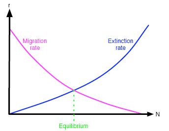
Figure 1: Migration and extinction curves for a typical island.
Slugs in equilibrium
If the number of species migrating to an island is equal to the number going extinct from the island, then the overall number of species does not change, that is, N is constant. In such a situation, we say that the number of species is in equilibrium. The equilibrium state of a system is very important. If two tug-of-war teams are in equilibrium, then neither team can move and neither will win (or lose). If the force your mass exerts on your chair due to gravity (i.e. your weight) is in equilibrium with the force the chair exerts on you, then you can continue reading this article in peace. If not, your chair will collapse under you or you will rocket off into space. Equilibrium is important. Systems left alone to evolve will tend toward equilibrium (although they might not stay there), just like a hot cup of coffee will gradually cool down to the temperature of the room (it does so by giving some of its heat energy to the room, heating it very slightly).
Figure 1 shows the equilibrium position for a typical island. Equilibrium occurs where the two curves cross — when the two rates are equal. In general, how are the two curves affected by the size of the island, and by the distance of the island from other islands? For the sake of this discussion, we will consider only the distance from a large, species-diverse island.
Slippery slopes
First, we check that the extinction curve really does have the shape shown in figure 1. As the number of species present increases, pressures due to climate, disease and sheer bad luck act on more species, and so the rate of extinction increases. In other words, the extinction rate curve has a positive gradient, or slope.
In terms of the effect of island size, a smaller island will have fewer resources to offer and competition for these and for the limited space available will increase the extinction rate. That is, the extinction rate curve for a smaller island lies above that of a larger one. Moreover, both extinction rates are zero when N=0 (if no species are on the island, then none can become extinct). It follows from these last two facts that the extinction rate curves for smaller islands have larger gradients; steeper slopes, as shown in figure 2.
The migration curves have negative slope for the following reason. If there is a large number of species in an island — that is, if N is large — then there are fewer new species which can migrate to the island from any neighbouring island. Since bigger islands will generally offer greater resources, a newly-arrived organism is more likely to become established in a larger island than in a smaller one. This implies that the migration curve for a larger island lies above that of a smaller island. In fact, it also has steeper slope because when N is equal to the number Nmax of all the species in the entire world, then the migration rate is zero for all islands: if all possible species are already present on an island, then no new ones can establish themselves. This means that all migration curves meet at the point (Nmax,0) and so must have different slopes — as shown in figure 2.
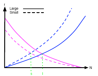
Figure 2: The effect of island size on the typical migration and extinction curves
The effects of distance from other islands can also be determined. Being close to other islands does not affect the extinction rate because in terms of extinctions what happens on one island is independent of what happens on others. However, the more isolated an island is from its neighbours, the less likely is it that new species will turn up, because only the hardiest of organisms can cover the large distances. Thus the migration rate is influenced by proximity to a significant pool of species on a nearby large island, with migration rate increasing for nearer islands, as shown in figure 3.
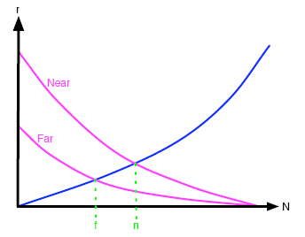
Figure 3: The effect of distance on the typical migration and extinction curves.
Species mix-up
We now turn to the equilibrium points marked l, s, f, n on figures 2 and 3. Remember that the systems tend towards equilibrium, so it is worth investigating these points. Firstly when comparing islands of different sizes, we note that the equilibrium value of N for larger islands, l, is larger than that for smaller islands, s. In other words, the number of established species on islands at equilibrium increases with island size. In figure 3, the equilibrium point f for those islands far from another larger, species-diverse island is smaller than that for nearer islands, n. In other words, the number of established species on islands at equilibrium decreases with distance from a larger island.
But we can say even more. Consider two islands of equal size, both at equilibrium and both satellites to a large island, but one quite close and the other further away. By looking at figure 3, we can see that the equilibrium extinction rate of the closer island is greater than that of the further island. Then, because organisms on the closer island are going extinct at a greater rate than on the further island, the species composition on the closer island will also change more rapidly than that on the more distant island, when they are both at equilibrium.
Now suppose that the effect of island size on the migration curve is quite small so that the dashed pink line of figure 2 is very close to the solid pink line. Since the point at which the dashed lines meet gives the equilibrium extinction and migration rates of the smaller island, then in this case we can say that those rates are higher than for the larger island (given by where the solid lines meet). For the same reason we just discussed, the smaller island would then be expected to have a more rapidly changing composition of species than the larger island. It should be quite easy for our sluggy friend to notice this effect because smaller islands have fewer species at equilibrium (s is smaller than l).
Phenotypic development
Slugs may develop the strangest phenotypes.
So much for species arriving at and dying out from an island. However, over long periods of time, the island's environment will affect the development of each species. After a significant passage of time a species may display a wide range of outward characteristics. For example, snafflegrass may grow leaves of different size in different islands. Each distinct set of observable characteristics is known as a phenotype. What can graphical methods tell us about how phenotypes emerge?
Central to this discussion is the idea of fitness. Not concerned with how fast a species can run, or how fast they can slime in the case of slugs, rather fitness as a measure of how able an individual of a certain species is to pass on its genes to the next generation, within a given environment. We won't worry too much about the exact definition of fitness, but it probably means something like the expected number of offspring at each generation.
Gus's world
Let us consider a sample individual of a sample species, and call him Gus. Suppose Gus's fitness in a certain environment suggests that he will have 10 surviving offspring. Presumably his offspring will have very similar fitness, so Gus can expect to have 100 grandchildren and his genetic legacy is quite large. But if he can only be expected to have 1 offspring, then he will only have one grandchild — a significantly weaker genetic influence on the population by the second generation. As the generations pass, this effect becomes even more significant.
Let us consider Gus's species in Gus's island, and suppose that there are two distinct environments in this island. Perhaps Gus is an insect which lives on grasses, and prefers to eat snafflegrass, but if pushed will eat urgleleaf. Let fitness be represented by a number F. The following analysis can be extended to variable fitnesses and to more than two environments.

Snafflegrass or urgleleaf?
Let us suppose that Gus spends a proportion p of his time hanging out in the snafflegrass. If he spent half of his time there, p would be 0.5; if three quarters then 0.75. Measured as a proportion of his whole time, p will be a number between 0 and 1. Since Gus prefers the snafflegrass he spends most of his time there, and so p will be close to 1. The remaining time he spends with the urgleleaf, which must represent a proportion 1-p of his total time. Let Gus's fitness in the snafflegrass (the expected number of descendants if he does his breeding there) be F1 and that in the urgleleaf be F2. Then his total fitness F is given by
You can see that this formula is correct by trying extreme values of the parameters and variables (a useful trick). If Gus is equally fit in both the snafflegrass and the urgleleaf — if F1 = F2 — then the formula reads
which is obviously correct. On the other hand, if he spends all his time in the snaffle grass — if p = 1 — then the formula becomes
which again is what we expect. If you try some other extreme values, such as p = 0, then you can convince yourself that we have the correct formula, that none other will do.
The overall fitness F and the fitnesses F1 and F2 are personal attributes of Gus: other members of his species may have different fitness values. The number p, however, is the same for all members of his species, as they all have more or less the same taste when it comes to grass.
We will make the (quite reasonable) assumption that those individuals of Gus's species less well-fitted to their environment tend to die out, and so the species as a whole increases its fitness (if it doesn't go extinct). Over time, this might mean the development of a new phenotype. Hence to study the emergence of phenotypes, our slug mathematician will want to maximise the equation
in other words find those values of F1 and F2 that make F as large as possible.
The shape of fitness
It's time we looked at some graphs. Suppose we mark each individual in Gus's species as a point on the plane: its co-ordinates are (x,y), where x is its fitness F1 and y is its fitness F2. Now all the biologically possible individuals together form a set of points on the plane called the fitness set.
A fitness set for two very similar environments might look like the one shown in figure 4. Those individuals with large F1 and small F2 represent a possible emergence of a phenotype specialised for environment 1, and vice versa. Most individuals can survive in both environments because of the similarities between them. The individual at point A is neither a specialist for environment 1 nor for environment 2 — she is an intermediate individual. But she still stands a good chance of surviving in either environment because for her both F1 and F2 are quite high. Such intermediate individuals are therefore likely to survive and reproduce. This means that the emergence of distinct phenotypes is unlikely because such a variety of individuals reproduces at each generation.
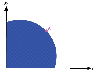
Figure 4: The fitness set for two similar environments
If on the other hand the environments are quite different, then the fitness set may look more like that in figure 5. Here, a clear tendency towards specialisation can be seen. The specialist at C is unlikely to be able to survive in the environment for which D is a specialist, and vice versa. Moreover, the unfortunate intermediate individual B is not well-fitted to either environment, and so is unlikely to produce a significant number of offspring. In this way, the genetic legacy of the specialists is far greater than that of the intermediates, and so two distinct phenotypes will emerge as the generations pass.
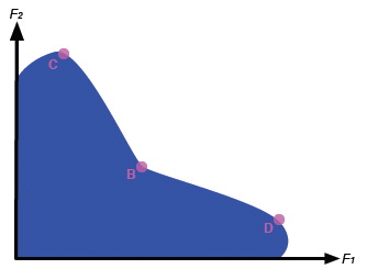
Figure 5: The fitness set for two dissimilar environments
More formally, consider our formula
We want to find those individuals that maximise their overall fitness F. Let's first look at all the individuals that have overall fitness F = F1p F2(1-p) = c, for some number c. Rearranging, we get
Writing this using the more conventional variables x and y instead of F1 and F2, and replacing c(1/(1-p)) and p/(1-p) by the letters a and b, this is y = a/xb. Since p is close to 1, b = p/(1-p) will be quite a large number. A bit of thought will convince you that such a curve looks like the shapes shown in figure 6 — they are similar to hyperbolae. If such a curve meets the fitness set, then there are individuals that do have overall fitness F=c.
Now let's increase c, the overall fitness, keeping p fixed. Each new curve will have a similar shape, but will be drawn further and further away from the axes, as shown in figure 6. If a curve for a particular c slices right through the fitness set in figure 5, then we could increase c: move the curve further away from the axes, and if it still intercepts the fitness set then we have increased F for biologically possibly individuals. You can probably see that you can repeat this process until you find a curve which only touches the fitness set at a single point: it is tangent to the fitness set. This process is shown in figure 7. What we find is that the specialist at D has maximal overall fitness.
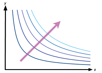
Figure 6: The curves for distinct values of the constant c. The arrow indicates increasing c.
If you have not had enough yet, figure out the shape of the curves for small p, and convince yourself that this will give the specialist at C as the one with maximal fitness.
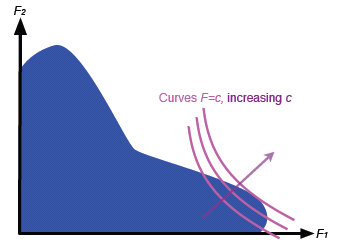
Figure 7: The process of finding the optimal individual.
So — a stick, a bit of sand and some basic graphical reasoning enabled our sluggy friend to get an overall picture of how species find a foothold and develop. He can easily test his conclusions against reality. Looking up from his scratching he might find a species with a great variety of mouth sizes, all the better to eat different sizes of urgleleaf leaves. This would correspond to the situation in figure 4. In another part of the island, he might see insects mimicking other insects which are distasteful to predators. Clearly, an insect which tried to mimic more than one other species at once — an intermediate mimic — would probably not be very convincing as either and be quickly eaten. This is the sorry individual B in figure 5.
But what about slug civilization? How will it develop in those places where it manages to take root again? How will its trade and commerce evolve? This is what we'll look at in the third and final part of this article, which will appear in the next issue of Plus.
About the author

Phil Wilson uses mathematics to understand how the skin of red blood cells works. The people he works with at the University of Tokyo hope that they can use this understanding to invent better ways of delivering medicine to the body. He is well-known in gastropod society for his pioneering work mentoring promising slug mathematicians.