Matrix: Simulating the world Part I - Particle models
Building models forms the core of many areas of scientific and engineering research. Essentially, a model is a representation of a complex system that has been simplified in different ways to help understand its behaviour. An aeronautical engineer, for example, might build a miniaturised physical model of a fighter plane to test in a wind tunnel. In modern times, more and more modelling is being performed by computers — running mathematical models at very high rates of calculations. A computer model of the flow of air over a supersonic wing is incredibly sophisticated, but it is based on very basic principles of program design and simulation. In this article, the first half of a two-part feature on model behaviour, we'll take a look at how simple computer models can be programmed to study some very interesting natural systems as well as focus on how a few scientists are using similar models in their own front-line research.
Getting started
Which way are they going? Find out how to simulate fish behaviour.
This is a hands-on introduction to mathematical modelling and computer simulation, but won't involve an in-depth lesson on programming itself. If you've never even looked at a program before, don't worry because all of the simulations can be watched as Java videos on this website too. If you have done a little bit of computer programming you might like to download all of the code used in this article and play around to see how you can improve or adapt it. The software used to write these simulations and produce the animations is called Processing, and is available in PC and Mac versions as a free download here. Processing has been released as a collaboration between computer scientists and artists, and is extremely easy to pick up and start using yourself. Have a look at their homepage for a list of all the different projects Processing has been used for around the world.
The essence of building a good model is to think how best to simplify a complex problem, to distil the crucial features of a system and leave out anything that might confuse the analysis of the model's behaviour. For example, a simple model of the trajectory of a bullet fired down a rifle range obviously needs to take into account the action of gravity, but could safely ignore the slight effects of air resistance. Air resistance in this case would be called a second-order effect. When modelling a different system, the lift produced by an aircraft wing, for example, the action of the air cannot be ignored but other factors could be left out. The trick is to find a balance between keeping your model as simple as possible so that you can understand its behaviour and see how changing one of the inputs affects the response of the whole system, without cutting out too much that might be important and so produce meaningless results.
All of the examples in this first article are what are known as particle models — they model the movement of individual points around space depending on various rules.
Gas molecules in a box
For our first model we'll write a very basic physics simulation of molecules of gas trapped in a box. To keep things nice and simple we'll only look at two dimensions — the particles are restricted to a square plane. The physics of this situation is easy — each particle continues in a straight line with the same direction and speed it started with, unless it hits one of the walls of the box. In this case, the molecule bounces off again, its direction changes accordingly, but its speed remains the same.
Like any movie, the animations in this article consist of a series of frames merging together to give the impression of fluid motion. The program's job is to calculate the position, direction and speed of each particle at each time step, based on the information from the previous step.
All the examples in this article store the data at every time step in an array, or a matrix as it is called in maths-speak. Each row of the matrix stores the necessary information on a different particle. In this gas example, the state of every particle is described by four numbers. Two of them give its (x,y) position in the plane. The other two describe the speed with which the particle moves in each of the two directions. They are called deltaX and deltaY (meaning "change in X position" and "change in Y position") and together they define the velocity of the particle. Thus the matrix in this case has four columns, and enough rows for all the particles. After every time-step of the simulation, the (x,y) position of each particle is updated depending on its velocity.
The structure of the program written to model this process is also fairly straight-forward. Have a look at the code and see if you can get at least the general gist of how it works.
The first thing that needs to be done is to define the most important parameters of the model, such as how many molecules to include, and the matrix that will store the information on the position and velocity of each particle.
Next, Processing demands that the simulation is set-up in terms of the size of the world, which is a square in this case, and frame-rate of the animation. After that the simulation is initialised. This is where we fill-in the data storage matrix with the necessary information on the starting position and velocity of each particle in turn. In this case we have chosen to scatter the particle randomly. Next, we have some code that draws the current state of the system, with a turquoise-coloured background and a red circle placed at the (x,y) location of every particle.
Finally, comes the core of the simulation itself, the update function. At every given time step, This function takes each particle in the matrix in turn and calculates whether its velocity would take it outside the boundaries of the box during this time step. If so, the particle velocity is changed accordingly and it bounces off the wall of the box, otherwise it moves forward by an amount given by its velocity vector (deltaX,deltaY). Thus, each particle now has a new position and possibly a new velocity vector and the matrix is updated with these new values.
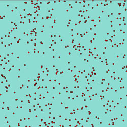
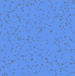
Model of gas molecules contained within a box. Click on the image to run a Java version of the simulation. You can restart the simulation by refreshing the window with [Ctrl]+[F5] (in Windows) or [z]+[R] (on a Mac). |
The entire program is set to loop so that after the particles have been updated the system is drawn again, then the particles updated once more, and so on until you stop the program. This happens so quickly on fast modern computers that the images flow together into a smooth animation of the gas molecules. The picture link on the right opens up a Java version of this program, so you can see it work even if you haven't installed the Processing software.
You'll notice that there are two main problems with this overly-simplistic model. Firstly, our program uses only integer values for deltaX and deltaY. This means that there aren't many different directions the particles can move in. Some of the particles can be seen moving perfectly horizontally or vertically as they bounce straight back and forth between two sides. Secondly, this code includes no interaction between the molecules — they never collide with each other and simply bounce around inside the box in a completely predictable way. Periodically all the molecules converge back into a tight cluster in the middle before dispersing outwards again like at the start. This obviously would never happen with the air molecules inside the room you're sat in — they constantly knock into each other to produce very unpredictable motion.
If you already know a bit about computer programming, you might want to take this simple example as your starting point and make it much more sophisticated and realistic. Some tips on how to do this are given at the end of the program file.We'll now move on to another example of modelling motion; this time there are slightly more complicated rules governing how the particles interact with each other.
Bird flocking
The system we'll model is that of a flock of birds; not moving completely independently like the first example but with each particle responding to the motion of others. We'll use the same standard structure as the gas program: first defining the parameters and setting up the world size, initialising the starting positions and velocities of all the particles, and next looping around functions that display the current state of the system and then execute the rules to calculate how the system changes over the next time-step.
In the first example we wanted to simulate the motion of particles trapped inside an enclosed space. This time, however, we're interested in looking into how birds flock when flying in the open. We don't want the world to have any edges because the simulation won't behave properly around these artificial features. A common trick in modelling is to define the world space so that if a particle moves off the left-hand side it re-appears on the right, and likewise with the top and bottom edges. The top and bottom have been rolled round so that they join together into a tube, and then the left and right ends have been bent round to join together as well — effectively we have remoulded the world into the surface of a doughnut (a torus in maths-speak).
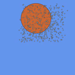
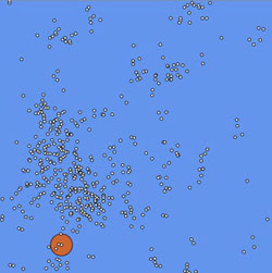 Model of bird flocking — a set of simple rules operate on the motion of each particle to determine how it interacts with other birds. The orange circle displays the eyeSight range. Click on the image to run a Java version of the simulation. You can restart the simulation by refreshing the window with [Ctrl]+[F5] (in Windows) or [z]+[R] (on a Mac) |
The second advance in this model is that instead of the particles continuing in a straight line, the birds interact with each other and change their direction of flight depending on their neighbours. At every time step, the program takes each bird in turn, calculates the average flight direction of any other birds within a chosen range, and gets the bird to steer into this direction. This field-of-view range is displayed as an orange circle around one randomly-selected bird. In the program the variable that stores its value is called eyeSight. Take a look through the computer code here to pick up the general gist of how the program works, and then try a few runs of the simulation with the image link on the left.
Almost immediately the initially-random motion of the birds has transformed into ordered behaviour. Great clumps of birds have spontaneously organised themselves into all flying in roughly the same direction. Lone birds get attracted into the flocks, and occasionally when two great groups stray too close to each other individual birds peel away to join the other flock as the two clouds smoothly merge together, waver for a short while and then settle on a new group heading. Compare this modelled behaviour to the dynamics of real bird flocks.
At the time of writing this there is a wonderful advert being run on British television for a certain hops-based beverage, showing the mesmerising flocking of swallows at dusk, and ending with the tag-line "Belong". Follow the image link on the right to watch this advert through YouTube, or if it has been removed you'll have no trouble finding other videos of bird flocking.
 Click on the image to watch an advertisement showing large-scale bird flocking, hosted by YouTube. |
This motion appears exquisitely choreographed, with every individual seemingly knowing exactly where it needs to fly next and great streams of birds co-ordinated to all smoothly change direction together. But within a flock no one bird is the leader; there is no master plan and all decisions are made by the group dynamics alone. All of the mesmerising complexity of thousands of flocking birds arises out of the very simple rules that each individual operates by, without any knowledge of what the rest of the group is doing beyond its most immediate neighbours. This is known as bottom-up control, and is an example of emergence — very complex group behaviour arising out of individuals interacting through simple rules. Lots of animals use this kind of "swarm intelligence", including bees, wasps, ants and termites.
But these simple rules underlying flocking behaviour can in unusual circumstances also produce distinctly-unintelligent behaviour. I've not had the opportunity to try this myself, but I've been reliably informed, by a friend of a friend, of an amusing trick you can pull off with a flock of sheep. If you run suddenly at the sheep they'll naturally try to move away from the perceived threat, whilst still operating their rules that it's safest to keep as close as possible to your neighbours and run in the same direction. But if you keep running slightly faster than the sheep, you overtake them and pass right through the middle of the flock and are now running in front. The group dynamics have taken over from the initial individual decision to run away from an aggressor, and you end up having the entire flock following behind you, rather than trying to escape!
Bats and eagles
If you download the Processing software and the programming code for this model you can tweak certain features of the model to see how it affects the overall behaviour of the group. For example, how far each bird can see, the eyeSight variable, is a very important parameter. In our program above its value is set to 20 (ie. the orange circle showing the visual field of one bird has a radius of 20 units), but this parameter can be set to any value you like. Let's take a look at two different scenarios: the "blind as a bat" case where eyeSight equals 1, and the "eagle eyes" case where the birds' eyeSight equals 100 and they can see right across the map. Both of these simulations can be watched by clicking the two links below.
Blind as a bat, eyeSight = 1 |
Eagle eyes, eyeSight = 100 |
|
Click on the images to see a Java version of the simulations. |
|
In the first scenario the birds do not interact with each other at all, and are effectively the same as gas molecules whizzing randomly around the world space. In the other case, there is too much long-distance communication as birds respond to the flight direction of individuals right on the other side of the group. The group behaviour solidifies very quickly into a uniform rigid movement. In both situations all the complex flocking behaviour has been lost, due to either too little or too much interaction. The system output is said to be very sensitive to this particular parameter. There is a kind of phase-transition between the gas-like and solid-like behaviour, both equally dead in terms of interesting dynamics, as the natural-looking emergent behaviour only arises when the value of eyeSight is somewhere in between these two extremes.
Jiggling along
Another important modelling parameter is what we call the random jiggle (denoted randomJiggle in the program). It takes account of the fact that a bird's assessment of the average flight direction of near-by birds is not always dead-accurate. When the program updates each bird's direction at a given time step it adjusts it by some random angle that lies within a range given by the random jiggle variable. For random jiggle values less than about 10° the flock eventually settles down into uniform motion in a single direction. And with randomJiggle set to 180° the system effectively becomes a simulation of the Brownian motion of dust motes.
As in the gas molecule example, there are several ways in which this model can be made more natural. Some tips on this are given at the end of the program file.
Simplicity versus speed
A crucial factor when writing a model is the efficiency of the algorithm used. The word "algorithm" descends from the name of the Arabic mathematician al-Khowarazmi, but has come to mean "a series of instructions followed to complete a task". The algorithm used in our bird flocking example here is in fact probably not very natural. A real bird doesn't actually log the position of every other bird, calculate the hypotenuse distance between itself and them all, select only those closer than exactly 5 m, and then steer towards the arithmetic mean of their headings. These steps were chosen for the model because they are easy to follow and do produce the desired result. It is quite a long-handed method, however, and requires calculating the distance from one bird to every other, for each bird in turn, and every time-step. Even on a fast desktop computer, the simulation chugs through achingly slowly for bird numbers greater than about 500.
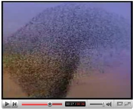
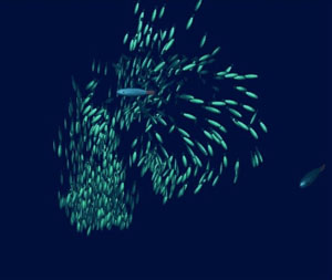
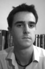
Iain CouzinIain is an expert on animal behaviour based at both Princeton University and University of Oxford. He writes computer models of the group dynamics of everything from locusts to fish and birds. His research is discovering startling features of how groups of animals make decisions collectively, and even helping agencies in Africa control lethal swarms of locusts. Most recently, Iain has been focussing on how groups respond to the approach of a predator. You can read more about Iain's work on his website. The image below shows a still from a video produced by one of his models that was used by the BBC in their documentary series "Predators".
Image courtesy BBC |
So when designing a model you also need to think about how to accomplish the task — whether you use an algorithm that is as fast as possible, or as close to the actual method used within the real system, or simply a method that may be inefficient but gets the job done. Often in programming it is a good idea to put the algorithm for a particular task in its own function, so that you can call upon it within the program whenever you need a particular calculation. (If you look at the bird flocking code, you will see that this has been done for the MeanHeading() function.)
If you wanted a simulation to run much quicker while you watch, you could break it down into two stages. The first runs through all the computer-hungry calculations, and saves the state of the system at each time-step as a separate matrix. So after running it for 1,000 time steps, say, you end up with a list of matrices like a stack of printed sheets — a three-dimensional matrix. Once the simulation has run through and all the information has been saved, the second stage is to simply display each time-step in turn (and without having to wait for all the calculations to process this time) — like flicking through the pages of the book of matrices to watch an animation.
We have focussed on this simple bird flocking simulation because it highlights important aspects of computer modelling, such as the structure of a computer program and writing algorithms and functions for particular tasks. Even with such a simple model, however, complex and very natural-looking group behaviour is produced. This is exactly the kind of computer model that animal researchers build to try and understand the flocking behaviour of birds or schooling of fish. For example, Dr. Iain Couzin (see the box above) uses computer models of large groups to help him understand animal behaviour. His models are based on exactly the same principles as the one we've looked at in this article and show the same stunning emergence of complexity; they are just more sophisticated, working in three dimensions (rather than our two-dimensional plane) and with a longer, more realistic, set of rules governing each individual's behaviour.
Gravitational Models
A further extension to this kind of particle motion modelling is to include effects that stretch right across the map. One obvious example of this is gravity — although it may become vanishingly slight, the gravitational influence of the Sun reaches over extremely long distances. To build a simple gravitational model using Processing you could draw a small circle in the centre of the screen as the Sun, and write a function to calculate the distance and direction to the Sun from any other point. From this you can calculate the gravitational force experienced and thus change in velocity of any particle in your modelled universe. Initialise the simulation with planets placed at random positions with random velocities and animate their arcing motion around the Sun, their position in the next time-step determined by the current gravitational force and velocity. You can also modify the program so that each planet leaves behind an orbital trail. (Remove the background command in the draw() function BY 'commenting it out' with // at the beginning of the line).
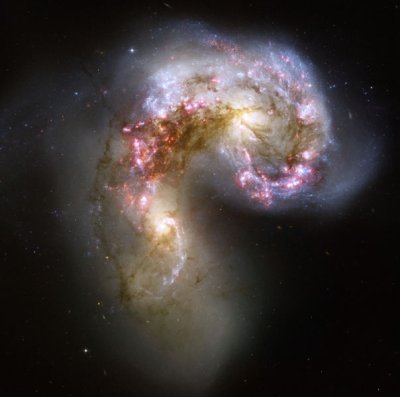
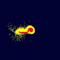
Billions of stars were formed during the collision of the Antennae galaxies. Find out more about modelling galaxy collisions below. This image was taken by the Hubble Space Telescope and appears courtesy NASA.
For a representation of the solar system you'd need to carefully work out the velocity that produces a circular orbit for each planet. Including only the Sun's gravity, by far the dominant force in the solar system, produces a model accurate to a first approximation. But the gas giant Jupiter exerts a noticeable influence on other planets, and so a more accurate model would include such second-order effects. To make the orbit of Mercury agree perfectly with observations, you'd have to add a further level of complexity and include Einstein's theory of relativity as this is more accurate than Newton's laws of gravity in certain situations. Again, the trick of modelling is to think cleverly about the minimum amount of detail you need to include — the Apollo program landed men on the Moon with a simple Newtonian gravity model and ignoring everything other than the influence of Earth and its satellite.
Modelling the dynamics of larger gravitational systems, where all particles interact with all others, becomes extremely "computationally expensive" — requiring enormous numbers of calculations on very fast computers. But such numerical simulations are crucial for many researchers. For example, the box below focuses on the work of two leading researchers, looking at events billions of years in the past and future: the world-shattering impact that is thought to have created the Moon and how the immense gravitational pulls of our own galaxy and our nearest neighbour will tear each other apart in billions of years to come.
Robin CanupRobin is a space scientist at Southwest Research Institute in Texas. She is interested in how the Moon formed, and tests the theory that it was born out of a "big splat" event right at the beginning of the solar system, when the young Earth collided with a smaller primordial planet. Her computer models calculate what happens as the whole Earth is melted by the heat of the impact, and a huge amount of rock is thrown up into space, much of it eventually coalescing into an orbiting satellite, the Moon. You can read more about Robin's work on her website. |
 Click image to link to an animation. |
John DubinskiJohn is an astrophysicist at Toronto University studying the dynamics of whole galaxies. Our galaxy, the Milky Way, and our spiral galactic neighbour called Andromeda are gravitationally attracting one another — effectively falling towards each other at 500,000 km/hr. John has used a supercomputer to model the time about 3 billion years in the future when these two huge
galaxies will begin to merge, tearing off great swathes of stars as the two rip through each other. Amazingly, despite all this disruption the gaps between individual stars will still be so great that none will actually collide. The fate of our Sun is uncertain, but it will either be ejected out into the dark void of intergalactic space, or plunge into the dense core of the merging galaxies. You
can read more about this at John's website, or watch movies by following the link below, including one of the view in Earth's night sky. |
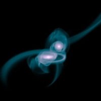 Click image to link to an animation. |
In the second article of this series we'll move on from particle-based simulations to look at so-called Cellular Automata models.
About the author
Lewis Dartnell read Biological Sciences at Queen's College, Oxford. He is now on a four-year combined MRes-PhD program in Modelling Biological Complexity at University College London's Centre for multidisciplinary science, Centre for Mathematics & Physics in the Life Sciences and Experimental Biology (CoMPLEX). He is researching in the field of astrobiology — using computer models of the radiation levels on Mars to predict where life could possibly be surviving near the surface, as recently reported in the news.
He has won four national communication prizes, including in the Daily Telegraph/BASF Young Science Writer Awards. His popular science book, Life in the Universe: A Beginner's Guide, is out in March 2007. You can read more of Lewis' work at his website.