Restoring profanity
In the late 14th century Michel Menschein, a wealthy Viennese cloth merchant, commissioned local artists to paint a series of frescoes on the walls of his banqueting hall. The paintings depicted a cycle of songs by Neidhart von Reuental, a 13th century minnesinger, who was particularly fond of satirising the erotic relationships between knights and peasant maidens. While the steamy subject matter doubtlessly enlivened many of Menschein's dinner parties, it didn't go down so well with subsequent occupiers. When the banqueting hall came into the possession of a Catholic priest in the late 16th century, the frescoes were painted over, and remained hidden for 300 years, until their chance re-discovery in 1979. They now represent the oldest instance of non-religious wall painting in Vienna, and provide a unique glimpse into medieval humour and society.
But the centuries under layers of paint and plaster, as well as the laborious process of exposure, took their toll on the frescoes. All were damaged and some were almost completely destroyed. A restoration effort, led by Wolfgang Baatz of the Viennese Academy of Fine Arts, was duly taken up, and it was supported by a group of mathematicians, including Peter A. Markowich, Massimo Fornasier and myself. It was an unusual collaboration, perhaps, but one which makes a lot of sense in this age of digital imagery. Digital photographs of the frescoes are essentially mathematical objects, and this puts the vast toolbox of mathematics at the restorers' fingertips.
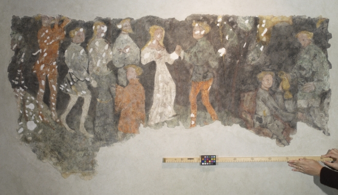
Figure 1: Part of the Neidhart frescoes. Image courtesy Andrea Baczynski.
Number pictures
A digital image is a mathematical object because it is an array of numbers. Jpeg photographs created with digital cameras are rectangular objects consisting of a finite number of image points (called pixels). The image content is described by numerical values corresponding to the pixels' colour. To make things easier, we'll concentrate on grey value images. Here every pixel comes with a number between 0 (black) and 255 (white). The mathematical representation of a digital grey value image is a so-called image function $u$, defined on a two-dimensional (in general rectangular) image domain. The function value $u(x, y)$ denotes the grey value of the image at the image point $(x, y)$ in the image domain. Figure 2 visualises the connection between the digital image and its image function.
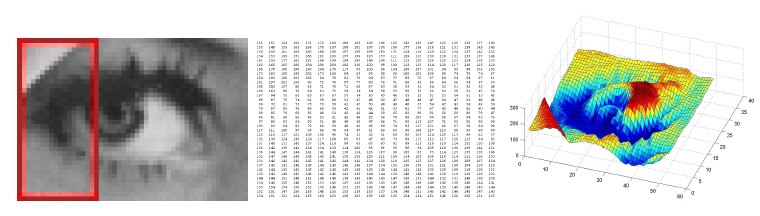
Figure 2: Digital image versus image function: The image on the left shows a zoom into a digital photograph where the image pixels (small squares) are clearly visible; in the middle the grey values of the red selection in the digital photograph are displayed in a matrix form; on the right the image function of the digital photograph is shown, with the grey value u(x, y) plotted as the height over the (x, y)-plane.
In a damaged image the value of the function $u(x,y)$ is unknown for a number of points $(x,y).$ The mathematical challenge is to use the information from surrounding pixels in an optimal way, to guess what the missing values should be. A prime candidate for completing this guesswork is an equation from an area which, on the face of it, has nothing to do with images, let alone art.
Heat flow
The heat equation
Assuming, for simplicity, that the rod is flat and two-dimensional, the rate of change of temperature over time at a point $(x,y)$ is given by the partial derivative $\frac{\partial T(x,y,t)}{\partial t}$ of the function $T$ with respect to time. Fourier's heat equation reads $$\frac{\partial T(x,y,t)}{\partial t} = k \left( \frac{\partial^2 T(x,y,t)}{\partial x^2} + \frac{\partial^2 T(x,y,t)}{\partial y^2}\right),$$ where $$\frac{\partial^2 T(x,y,t)}{\partial x^2} \; \mbox{and} \; \frac{\partial^2 T(x,y,t)}{\partial y^2}$$ are the second order partial derivatives of $T$ with respect to $x$ and $y$ respectively, and where $k$ is the thermal conductivity of the metal, a constant describing its ability to conduct heat.
In the early nineteenth century the mathematician Joseph Fourier became interested in the way heat propagates in solid bodies, for example metal rods: if you heat up one end of it at time zero, what will the temperature $T(p,t)$ be at any point $p$ of the rod at time $t$?
Fourier realised that a relatively simple equation describes the way temperature changes at a given point on the rod in an instant of time. From this information on the rate of change of temperature over time, and from information on the initial temperature conditions at time zero, it's then possible to work out the function $T(p,t)$. Mathematically, rates of change are described in terms of derivatives of functions, and the heat equation is what is known as a partial differential equation. See the box on the right for more detail on the heat equation.
Diffusing images
Fourier's equation, also known as the diffusion equation, works not just for the propagation of heat, but versions of it can be applied in many situations where the concentration $u(x,y,t)$ of some quantity at point $(x,y)$ changes over time $t$. And this is where the application to images comes in. As an example, let's start with a function $u$ which randomly allocates a grey value $u(x,y)$ to point $(x,y)$ on our rectangular image, giving the image on the left-hand side of figure 3. We can now let the diffusion equation do its work on the image: rather than heat, it is now the information from the various pixels that "migrates" across the image over time, changing each grey value using the information from surrounding ones. The image on the right shows the solution for $u$ at time $t=10.$ The content of the initial random distribution (which may also be identified with white noise) is smeared out by the application of the diffusion operator.
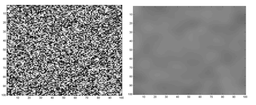
Figure 3: In the image on the left grey values have been randomly allocated to the pixels. The image on the right shows the solution to the diffusion equation for t = 10.
What happens now if we solve the diffusion equation for the image function of a real image? In figure 4 you can see the answer at time $t = 10$ for an image of the sculpture V Tiempo de la VI Sinfonia Pastoral de Beethoven by Leone Tomassi, which stands in the botanical garden of Buenos Aires. The result is not really surprising. It's more or less the same diffusive effect as for our random function in figure 3.
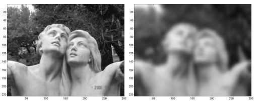
Figure 4: The diffusion equation applied to a digital image of a sculpture.
If we add some noise to the image before feeding it to the equation, we obtain the right image in figure 5 (the solution $u$ for $t=2$ to the diffusion equation). Now we might get an idea of the use of the smearing effect, namely the elimination of noise in images.
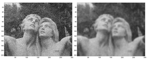
Figure 5: The diffusion equation applied to a noisy image of the sculpture.
But let's return to the task of repairing a damaged image. Consider figure 6, where several small holes have been cut into the image. It turns out that we can rescue it using a slightly modified diffusion equation. Roughly speaking, we now only solve the diffusion equation inside the black holes in the sculpture photograph, using the grey values from the surrounding of the holes as an input to the equation. In other words, the grey values inside the holes are constructed by "averaging" the grey values located around the holes. This process is called inpainting. The right image in figure 6 shows the result.

Figure 6: The diffusion equation applied to a damaged image.
The process of inpainting using the diffusion equation is just a first naive approach to the challenge of completing damaged images. Several more sophisticated approaches involving partial differential equations have been proposed in the last eight years. Among them is inpainting using a so-called total variation flow (TV), instead of the pure diffusion process. While the pure diffusion process equally diffuses all the image content, also edges in the image which indicate the boundary between regions of different colours, the TV flow preserves edges in an image and continues them into the damaged parts. An example of the application of a partial differential equation containing a modified TV flow to a damaged image is shown in figure 7.
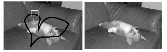
Figure 7: A modified total variation flow applied to a damaged image. Edges in the image are preserved.
Figure 8 shows a zoom of the damaged image in figure 7, and compares the result from inpainting using a total variation flow to that from a diffusion-like process. Clearly it is worth to investigate more sophisticated approaches like the total variation flow for these tasks.
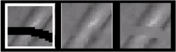
Figure 8: From left to right — zooming in on the white rectangle in figure 7, the result using a total variation flow, and the result using pure diffusion.
The Neidhart frescoes and beyond
A first approach to the restoration of the Neidhart frescoes is shown in figures 9, 10 and 11. Here the mathematicians first used a technique known as Cahn-Hilliard inpainting, which is based on a differential equation from material science, the Cahn-Hilliard equation. Traditionally, the equation is used to model a process called phase separation, in which a fluid mixture spontaneously separates into its two pure components. This occurs, for example, in metal alloys. In inpainting, this equation is used to reconstruct the binary (black and white) structure of an image. In a second step the respective grey values are filled into the missing parts using both the reconstructed binary structure and TV inpainting. (You can see a movie of the Cahn-Hilliard equation in action.)
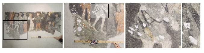
Figure 9: Zooming in on a damaged part of a Neidhart fresco.
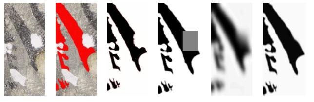
Figure 10: A specific structure in the fresco is selected and then reconstructed using Cahn-Hilliard inpainting for black and white images. From left to right: the original image; the relevant structure is identified; the structure is binarised (turned into a black and white image); the missing domain is identified (grey rectangle); the image structure is diffused into the missing domain, the structure is sharpened.
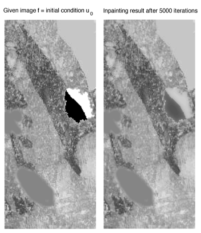
Figure 11: Based on the result gained from the structure reconstruction in figure 10, TV inpainting is used to fill the suitable grey values into the hole.
And here is an image of the fresco shown in figure 1 after the restoration.
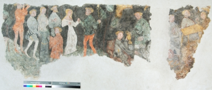
Figure 12: The restored fresco. Image courtesy Wolfgang Baatz.
To be fair, in the case of the Neidhart frescoes, the role of mathematics was limited — it was the mathematicians who learned from the restorers, rather than the other way around, and the mathematical approach served mostly as a rough inspiration. However, the collaboration helped to perfect existing mathematical techniques and inspired new ones. In future projects, mathematics will no doubt start pulling its full weight. What's more, applications of inpainting go far beyond the restoration of art. Ever since the pioneering works of Masnou and Morel in 1998 and Marcelo Bertalmio et al. in 2000, it has found wide applications in image processing in a wider sense. These include applications in computer vision, the use of inpainting as an artist's tool, and even medical applications. Diagnostic imaging, for example using PET (positron emission tomography) scans, often suffers from incomplete data and from noise added in the process of recording. In this case total variation-like approaches are used to pre-process the images.
About the author
Carola-Bibiane Schönlieb is a PhD student in the Applied Partial Differential Equations Research Group at the University of Cambridge, led by P.A. Markowich. She is working on her thesis on modern PDE techniques for image inpainting, which involves studying partial differential equations and their application in digital image restoration. She is concerned both with analytic properties of these equations, as well as their efficient numerical solution. The fresco project arose during the first two years of her PhD, which she spent at the University of Vienna. This project posed a very challenging task to her and the rest of the mathematical team and was one of the main motivations to work on the development of effective models for image restoration using partial differential equations.
The work described in this article is funded and supported by the Vienna Science and Technology Fund (WWTF) Fife Senses Call 2006 (project number CI06 003), by the Austrian Research Promotion Agency (FFG)(project number 813610), and by King Abdullah University of Science and Technology (KAUST) (award no. KUK- I1-007-43.)