Looking out for number one
So, here's a challenge. Go and look up some numbers. A whole variety of naturally-occuring numbers will do. Try the lengths of some of the world's rivers, or the cost of gas bills in Moldova; try the population sizes in Peruvian provinces, or even the figures in Bill Clinton's tax return. Then, when you have a sample of numbers, look at their first digits (ignoring any leading zeroes). Count how many numbers begin with 1, how many begin with 2, how many begin with 3, and so on - what do you find?
You might expect that there would be roughly the same number of numbers beginning with each different digit: that the proportion of numbers beginning with any given digit would be roughly 1/9. However, in very many cases, you'd be wrong!
Surprisingly, for many kinds of data, the distribution of first digits is highly skewed, with 1 being the most common digit and 9 the least common. In fact, a precise mathematical relationship seems to hold: the expected proportion of numbers beginning with the leading digit n is $\log_{10}((n+1)/n)$.
This relationship, shown in the graph of Figure 1 and known as Benford's Law, is becoming more and more useful as we understand it better. But how was it discovered, and why on earth should it be true?
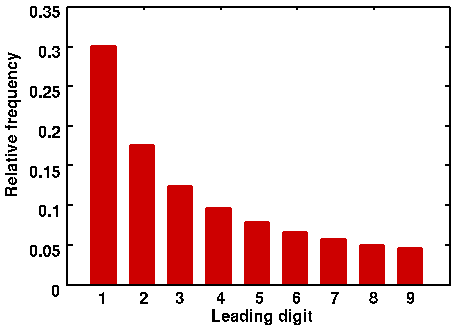
Figure 1: The proportional frequency of each leading digit predicted by Benford's Law.
Newcomb's Discovery
The first person to notice this phenomenon was Simon Newcomb, a mathematician and astronomer. One day, Newcomb was using a book of logarithms for some calculations. He noticed that the pages of the book became more tatty the closer one was to the front. Why should this be? Apparently, people did more calculations using numbers that began with lower digits than with higher ones. Newcomb found a formula that matched his observations pretty well. He claimed that the percentage of numbers that start with the digit D should be $\log_{10}((D+1)/D)$.
Newcomb didn't provide any sort of explanation for his finding. He noted it as a curiosity, and in the face of a general lack of interest it was quickly forgotten. That was until 1938, when Frank Benford, a physicist at the general electric company, noticed the same pattern. Fascinated by this discovery, Benford set out to see exactly how well numbers from the real world corresponded to the law. He collected an enormous set of data including baseball statistics, areas of river catchments, and the addresses of the first 342 people listed in the book American Men of Science.
Benford observed that even using such a menagerie of data, the numbers were a good approximation to the law that Newcomb had discovered half a century before. About 30% began with 1, 18% with 2 and so on. His analysis was evidence for the existence of the law, but Benford, also, was unable to explain quite why this should be so.
The first step towards explaining this curious relationship was taken in 1961 by Roger Pinkham, a mathematician from New Jersey. Pinkham's argument was this. Suppose that there really is a law of digit frequencies. If so, then that law should be universal: whether you measure prices in Dollars, Dinar or Drakma, whether you measure lengths in cubits, inches or metres, the proportions of digit frequencies should be the same. In other words, Pinkham was saying that the distribution of digit frequencies should be "scale invariant".
Using this reasoning, Pinkham went on to be the first to show that Benford's law is scale invariant. Then he showed that if a law of digit frequencies is scale invariant then it has to be Benford's Law (see the proof below). The evidence was mounting that Benford's Law really does exist.
Our own experiment
Is it really that simple to find data confirming Benford's law? We looked at some data from three sources: fundamental physical constants and vapour pressures (both from the Handbook of Physics and Chemistry) and annual turnovers in pounds (from Kompass Business Statistics). We chose a random collection of statistics from each of these categories, and counted up the number of occurrences of each leading digit. We got the following results (Table 1):| Digit | Fundamental constants | Vapour pressures | Annual turnovers |
| 1 | 22 | 36 | 44 |
| 2 | 11 | 21 | 25 |
| 3 | 2 | 16 | 12 |
| 4 | 5 | 15 | 15 |
| 5 | 5 | 10 | 9 |
| 6 | 3 | 11 | 11 |
| 7 | 2 | 9 | 9 |
| 8 | 1 | 8 | 10 |
| 9 | 4 | 6 | 2 |
| Totals | 55 | 132 | 137 |
Figure 2 shows the results above expressed as relative frequencies and plotted against the expected frequencies predicted by Benford's law:
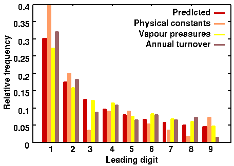
Figure 2
As you can see, there is a reasonable (but not perfect) correspondence with the digit frequency predictions made by Benford's law. However, as with any sampled statistics, we'd expect a better correspondence with the predicted values if we used a larger number of samples. In fact, if we calculate the relative frequencies of leading digits over all the sample data in table 1, we see that the frequencies approach the Benford predictions much more closely:
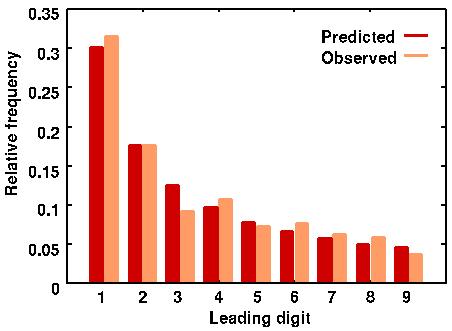
Figure 3
When does Benford rule?

Image: Adrienne Hart-Davis / DHD Photo Gallery
At this point, you might be tempted to revise the way you choose your lottery numbers: out go birthdays and in comes Benford. Will that make a difference?
Sadly, the answer is no. The outcome of the lottery is truly random, meaning that every possible lottery number has an equal chance of occurring. The leading-digit frequencies should therefore, in the long run, be in exact proportion to the number of lottery numbers starting with that digit.
On the other hand, consider Olympic 400m times in seconds. Not very many of these begin with 1! Similarly, think about the ages in years of politicians around the world: not many of these will begin with 1 either! Unlike the lottery, these data are not random: instead, they are highly constrained. The range of possibilities is too narrow to allow a law of digit frequencies to hold.
In other words, Benford's Law needs data that are neither totally random nor overly constrained, but rather lie somewhere in between. These data can be wide ranging, and are typically the result of several processes, with many influences. For example, the populations in towns and cities can range from tens or hundreds to thousands or millions, and are affected by a huge range of factors.
Tracking Down Fraud With Benford
Benford's Law is undoubtedly an interesting and surprising result, but what is its relevance? Well, the evidence has been mounting that financial data also fit Benford's Law. This turns out to be tremendously important if you're to detect (or commit!) fraud.
Dr Mark Nigrini, an accountancy professor from Dallas, has made use of this to great effect. If somebody tries to falsify, say, their tax return then invariably they will have to invent some data. When trying to do this, the tendency is for people to use too many numbers starting with digits in the mid range, 5,6,7 and not enough numbers starting with 1. This violation of Benford's Law sets the alarm bells ringing.
Dr Nigrini has devised computer software that will check how well some submitted data fits Benford's Law. This has proved incredibly successful. Recently the Brooklyn district attorney's office had handled seven major cases of fraud. Dr Nigrini's programme was able to pick out all seven cases. The software was also used to analyse Bill Clinton's tax return! Although it revealed that there were probably several rounded-off as opposed to exact figures, there was no indication of fraud.
This demonstrates a limitation of the Benford fraud-detection method. Often data can diverge from Benford's Law for perfectly innocent reasons. Sometimes figures cannot be given precisely, and so rounding off occurs, which can change the first digit of a number. Also, especially when dealing with prices, the figures 95 and 99 turn up anomalously often because of marketing strategies. In these cases use of Benford's Law could indicate fraud where no such thing has occured. Basically the method is not infallible.
However, the use of this remarkable rule is not restricted to hunting down fraud. There is already a system in use that can help to check computer systems for Y2K compliance. Using Benford's Law, it is possible to detect a significant change in a firm's figures between 1999 and 2000. Too much of a change could indicate that something is wrong.
Time, money and resources can be saved if computer systems are managed more efficiently. A team in Freiburg is working on the idea of allocating computer disk space according to Benford's Law.
Scientists in Belgium are working on whether or not Benford's Law can be used to detect irregularities in clinical trials. Meanwhile, the good correlation of population statistics with Benford's Law means that it can be used to verify demographic models.
Who knows where else this might prove useful? Dr Nigrini says "I forsee lots of uses for this stuff, but for me it's just fascinating in itself. For me, Benford is a great hero. His law is not magic but sometimes it seems like it".
Deriving Benford's Law
As Pinkham argued, the fact that we can find all kinds of data in the real world that seem to conform to Benford's Law suggest that this law must be scale invariant. Why? Because we can measure our data using a range of different scales (feet/metres, pounds/dollars, gallons/millilitres etc). If the the digit frequency law is true, it must be true for all of them (there's no reason why only one measurement scale, the one we happened to choose, should be the "right one").
So if there is a distribution law of first significant digits, it should hold no matter what units happen to have been used. The distribution of first significant digits should not change when every number is multiplied by a constant factor. In other words, any such law must be scale invariant.
Equally likely digits are not scale invariant
Most people have the intuition that each of the digits 1..9 are equally likely to appear as the first significant digits in any number. Let's suppose this is the case and see what happens with a set of accounts that are to be converted from sterling to the euro at the (fictional) rate of 2 euros to the pound.
It's fairly easy to work out what will happen by looking at each digit in turn. If the first significant digit is 1, then multiplying by 2 will yield a new first digit of 2 or 3 with equal probability. But if the first significant digit is 5 or 6 or 7 or 8 or 9 the new first digit must be 1. It turns out that in the new set of accounts, a first digit of 1 is 10 times more likely than any other first digit!
In the diagram below, the notation [a,b) means the range of numbers greater than or equal to a, but strictly less than b.
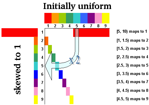
Figure 4: Equiprobable digit distribution changes with scaling
Our intuition has failed us - the original uniform distribution is now heavily skewed towards the digit 1. So if scale invariance is correct, the uniform distribution is the wrong answer.
Pinning down scale invariance
So what does scale invariance of the distribution of the first significant digit really mean? It means that if we multiply all our numbers by an arbitrary constant (as we do when we change from pounds to yen, or feet to metres), then the distribution of first digit frequencies should remain unchanged. \par Since we are interested in the distribution of first significant digits it makes sense to express numbers in scientific notation $x \times 10^n $ where $ 1 \le x < 10 $. This is possible for all numbers except zero. The first significant digit - $d$ is then simply the first digit of $x$. We can easily derive a scale invariant distribution for $d$ once we have found a scale invariant distribution for $x$. \par If a distribution for $x$ is scale-invariant, then the distribution of $y=\log_{10}x$ should remain unchanged when we {\em add} a constant value to $y$. Why? Because we would be {\em multiplying} $x$ by some constant $a$, and $\log_{10}ax = \log_{10}a + \log_{10}x = \log_{10}a + y$. \par Now, the only probability distribution on $y$ in $[0,1)$ that will remain unchanged after the addition of an arbitrary constant to $y$, is the uniform distribution. To convince yourself of this, think about the shape of the probability density function for the uniform distribution.
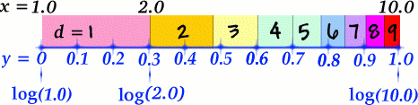
Figure 5
In figure 5, $y$ is uniformly distributed between $\log_{10}(1) = 0$ and $\log_{10}(10) = 1$. \par If we want to find the probability that $d$ is $1$ we have to evaluate \begin{eqnarray*} \\ Pr\big(d = 1\big) & = & Pr\big(1 \leq x < 2 \big)\\ \nonumber &= & Pr\big(0 \leq y < \log_{10}2 \big) \nonumber \end{eqnarray*} To find this we calculate the integral $$\int_{0}^{\log_{10}2}1 dy=\log_{10}2,$$ which is approximately $0.301$. In general \begin{eqnarray} Pr\big(d = n\big) & = & Pr\big(n \leq x < n+1 \big)\\ \nonumber & = & Pr\big( \log_{10}n \leq y < \log_{10}(n+1)\big) \nonumber \end{eqnarray} and this is given by \begin{eqnarray} \int_{\log_{10}n}^{\log_{10}(n+1)}1 dy & = & \log_{10}(n+1)-\log_{10}n \\ \nonumber & = & \log_{10}((n+1)/n) \nonumber \end{eqnarray} The expression $\log_{10}((n+1)/n)$ was exactly the formula given by Newcomb and later Benford for the proportion of numbers whose first digit is $n$. So, we can show that scale invariance for a distribution of first digit frequencies of $x$ implies that this distribution must be Benford's Law!
About the author

Jon Walthoe is presently a graduate student at the University of Sussex. As well as his graduate research, he is involved in the EPSRC-funded [ https://www.shu.ac.uk/schools/sci/pri/ ] Pupil Researcher Initiative.
After finishing his first degree at the University of Exeter, he opted out of Maths for a while. This involved working in local government among other things, and travelling in Latin America. When not doing his research, his favourite escape is sailing on the local waters in Brighton.
Comments
Anonymous
It might be expected, prima facie, that roughly the same number of surnames in a sample would begin with each letter of the Roman alphabet and that the proportions of surnames categorised by their initial letters would be approximately uniform and equal to 1/26.
However, for many kinds of alphabetic data, the distribution of initials is skewed. A mathematical relationship (known as Benford's law for numeric data) seems to hold when adapted to model alphabetic data.
See http://plus.maths.org/issue9/features/benford/ regarding numeric data.
Using logs with base 27, the expected proportion (P) of surnames beginning with any letter is P = log[(n+1)/n], where 0 < n < 27 is the alphabetic rank of the letter and the cumulative function of P = log[(n+1)/n] is Sum(P) = log(n+1).
This model indicates a probability that 33% of a sample of surnames will begin with either A or B and that 67% of the surnames in that sample can be expected to begin with one of the eight letters from A to H.
A generalised version of this law would not work for truly random sets of data. It would work best for data that are neither completely random nor overly constrained, but rather lie somewhere in between. These data could be wide ranging and would typically result from several processes with many influences.
Michael Mernagh, Cork, Ireland. February 17, 2011.
Anonymous
The better form of the Benford model for alphabetic data
Submitted by Michael Mernagh on June 1, 2011
As a general guideline for modelling alphabetic data, the cumulative form of the Benford frequency distribution seems more pleasing to the eye than the uncumulated form.
From: Michael Mernagh, Cork, Ireland.
Anonymous
This would fit in with my experience at school. We were housed based on our names. The four equally-sized houses were invariably split A-D,E-K,L-N and O-Z every year. Though I imagine this would not hold true in say the Arab World where about 90% of names begin with A so its probably not as universal as Benford's Law.
Anonymous
Brilliant article.
Needs to explain the distribution of random initial digits in the true random uniform distribution. The above just explains the "Benford" distribution in a uniform distribution that is multiplied by something.
Am I missing something?
Russ Abbott
Nice article, even though I'm coming across it 20 years after it was written. Here's another way to get a distribution that favors numbers starting with 1, then 2, etc.
Generate sets of random numbers according to the following scheme.
1. Select a range, 0 to n for some n.
2. Select k numbers in that range at random.
3. Repeat indefinitely.
How do you select n, the top of the range? Make that random in the range, say, 0 .. 99.
Any n will allow selection only of numbers from 0 .. n. So higher number, i.e., those greater than n will be excluded.
Given that we are performing this process multiple times, with a new n each time, when we aggregate all the random number collections it will include all numbers. But lower numbers will be more frequent than higher numbers because we select the top of the range to exclude larger numbers.
I haven't tried this experimentally. I wonder how close it would come to Benford's Law.
Russ Abbott
I did the experiment described in my previous comment and got a distribution that was similar to but not close enough to the expected one.
I generated 2 million numbers as follows. Let ranges_top = 999. Then generate a sequence of 2 million numbers based on this formula.
randint(1, randint(1, ranges_top))
In other words, to generate a number select a number at random between 1 and 999. Then select a number between 1 and that number.
The distribution was as follows (along with the expected results).
{1: (0.24, 0.30), 2: (0.18, 0.18), 3: (0.15, 0.12), 4: (0.12, 0.10), 5: (0.09, 0.08), 6: (0.08, 0.07), 7: (0.06, 0.06), 8: (0.05, 0.05), 9: (0.03, 0.05)}
That is, about 24% of my numbers began with 1 compared to an expected 30%, etc.
I did this experiment a number of times using Python's random number library. The results were all substantially the same.
Disappointing.
Is there anything known about the distribution I generated?
Russ Abbott
An additional level of randomness gets a lot closer to the theoretical distribution.
Generating 1 million numbers using the formula
randint(1, randint(1, randint(1, ranges_top))), where ranges_top is still 999,
produces this result.
{1: (0.31, 0.3), 2: (0.19, 0.18), 3: (0.13, 0.12), 4: (0.1, 0.1), 5: (0.08, 0.08), 6: (0.06, 0.07), 7: (0.05, 0.06), 8: (0.04, 0.05), 9: (0.04, 0.05)}
An additional level of randomness beyond three makes the result worse. So it's not a matter of converging to the result.