Add new comment

The mathematics of diseases

Back to the Epidemiology for beginners collection.

Diseases are a ubiquitous part of human life. Many, such as the common cold, have minor symptoms and are purely an annoyance; but others, such as Ebola or AIDS, fill us with dread. It is the unseen and seemingly unpredictable nature of diseases, infecting some individuals while others escape, that has gripped our imagination. From prehistory to the present day, diseases have been a source of fear and superstition. Over the past one hundred years, mathematics has been used to understand and predict the spread of diseases, relating important public-health questions to basic infection parameters. Here, we shall review the simplest of disease models and consider some of the more mathematical developments that have improved our understanding and predictive ability.

The mathematics of diseases is, of course, a data-driven subject. Although some purely theoretical work has been done, the key element in this field of research is being able to link mathematical models and data. Case reports from doctors provides us with one of the most detailed sources of biological data; we often know the number of weekly disease cases for a variety of communities over many decades. This data also contains the signature of social effects, such as changes in birth rate or the increased mixing rates during school terms. Therefore, a comprehensive picture of disease dynamics requires a variety of mathematical tools, from model creation to solving differential equations to statistical analysis.

Basic Models

Almost all mathematical models of diseases start from the same basic premise: that the population can be subdivided into a set of distinct classes, dependent upon their experience with respect to the disease. The most simple of these models classifies individuals as one of susceptible, infectious or recovered. This is termed the SIR model. Individuals are born into the susceptible class. Susceptible individuals have never come into contact with the disease and are able to catch the disease, after which they move into the infectious class. Infectious individuals spread the disease to susceptibles, and remain in the infectious class for a given period of time (the infectious period) before moving into the recovered class. Finally, individuals in the recovered class are assumed to be immune for life.

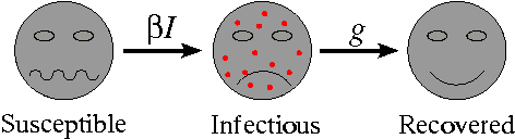
Movement rates between classes of the SIR model

We can make this description more mathematical by formulating a differential equation for the proportion of individuals in each class (the equations are shown at the end of the article). Computer simulations of this mathematical model agree well with mathematical theory, predicting decaying oscillations (you might want to compare this with the damped oscillations observed in a spring). Therefore, although initially this model shows large epidemics occurring at regular intervals, eventually the level of the disease reaches a constant value.

Damped oscillations of the SIR model

The Epidemiological Parameter R₀

Many interesting and useful results have been proved for the simple SIR model, but before we can explore this rich subject area, we need a further bit of Epidemiological notation. One fundamental parameter governs the spread of diseases, and is also related to the long term behaviour and the level of vaccination necessary for eradication. This parameter is called the basic reproductive ratio, $R_0$ . $R_0$ is defined by epidemiologists as "the average number of secondary cases caused by an infectious individual in a totally susceptible population". As such $R_0$ tells us about the initial rate of increase of the disease over a generation. When $R_0$ is greater than 1, the disease can enter a totally susceptible population and the number of cases will increase, whereas when $R_0$ is less than 1, the disease will always fail to spread. Therefore, in its simplest form $R_0$ tells us whether a population is at risk from a given disease.

The value of R₀ for some well-known diseases
Disease	R₀
AIDS	2 to 5
Smallpox	3 to 5
Measles	16 to 18
Malaria	> 100

The fit between cases and the SIR epidemic for bubonic plague and measles

A second use for $R_0$ is looking at the behaviour of a single epidemic outbreak. Consider the situation when a new strain of influenza enters a totally susceptible population. Simple intuition tells us that the disease will spread rapidly through the population, infecting a large proportion of the population in a very short time. It is therefore plausible to ignore births and deaths in the population and solely concentrate on the disease dynamics. For these short-term epidemics, initially the number of cases increases exponentially ( $I(t) \propto \exp [(R_0-1)t]$ ). However, as more of the population enters the recovered class and there are fewer susceptibles, the disease spreads less well and eventually the number of cases declines. Due to this decline not everyone will be infected before the disease dies out. By looking at the long-term behaviour of the SIR model, Kermack and McKendrick were able to predict the proportion of individuals ( $S_{\infty }$ ) who would escape the infection,

$S_{\infty } = \exp ([S_{\infty }-1] R_0).$

$[IMAGE: graph of S_\infty]$

A graphical method for calculating the percentage that escape infection

Although this expression cannot be evaluated analytically, by examining the two sides graphically (plotting $S_{\infty }$ and $\exp ([1-S_{\infty }] R_0)$ on the same graph) it is clear that as $R_0$ increases, fewer individuals escape the disease. Calculating $S_{\infty }$ numerically, when $R_0=2$ we find that $S_{\infty }$ is approximately $20\%$ , whereas when $R_0=5$ we get $S_{\infty }$ is approximately $0.7\%$ . Therefore, increasing $R_0$ has a dramatic effect on the proportion that escape the outbreak.

Finally, if we wish to model a disease that is endemic, that is, persists indefinitely in the population, our SIR model must also include births to replenish the level of susceptibles. In this case the long term behaviour of the disease can again be related to the parameter $R_0$ . The long-term proportion of susceptible individuals in the population, once the oscillations have died away, is given by

$S^{\star }= 1/R_0.$

Therefore, those diseases that spread the most rapidly have the fewest susceptible individuals. (It is interesting to note that the long-term level of infection, $I^{\star }$ , does not depend on the parameter $R_0$ , but instead is dependent on the birth rate and the infectious period.)

The concept behind vaccination is to reduce the proportion of susceptibles until the disease cannot survive. At the long-term level of susceptibles, $S^{\star }$ , each infectious individual on average causes one further secondary case. (If infectious individuals causes more or less than one case, then the level of infection would either rise or fall and the disease wouldn’t be stable.) Therefore, if we can reduce the number of susceptibles even further, so that the disease does less well, we can begin to eradicate the disease. The threshold level of vaccination ( $V_ T$ ) necessary to eradicate the disease is therefore

$V_ T = 1- S^{\star } = 1 - 1/R_0.$

It should now be clear why vaccination has allowed us to completely eradicate smallpox ( $R_0$ is approximately 4), whereas there are still cases of measles in Britain and the USA ( $R_0$ is approximately 17) despite mass vaccination, and why it is so very difficult to control malaria ( $R_0 >100$ ). It is important to realize that we don’t need to vaccinate everybody to eradicate a disease; by a process known as herd immunity, for each person that is vaccinated the risk of infection for the rest of the community decreases. Therefore vaccination does not just protect the individual, but also offers some protection to the whole community.

Foot and Mouth Disease

Incinerating cattle to help contain the spread of foot and mouth disease

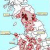
Recently there has been a great deal of attention focused on the spread of foot and mouth disease in the UK. This gives the mathematical modeller a prime opportunity to put all of the above theory into practice.

Foot and mouth is a disease of cattle, pigs, sheep and some other livestock, although fortunately not humans. It is common in areas of Africa and Asia, but it has been over 30 years since the last major outbreak in Britain. Foot and mouth spreads very rapidly and can be transmitted either by close contact within farms or at markets, or it can be wind-borne over much longer distances. In cattle and pigs the disease has disastrous consequences, and therefore modelling and understanding its spread is economically very important.

Foot and mouth disease can again be described by a simple SIR model. However, because its spread within a farm is so rapid, most models classify the entire farm as either susceptible, infectious or recovered. These farm-level models have an $R_0$ of around 50. Control of the disease is a difficult problem - very stringent measures need to be taken to overcome this large value of $R_0$ . Vaccination is not a useful policy as it only offers partial protection and must be repeated every 4-6 months. Instead, by destroying all infected animals and limiting the movement of livestock it is hoped that the transmission between farms can be reduced sufficiently that the disease will die out.

Computer-generated image of the foot and mouth virus

Complications

The theory outlined here has only scratched the surface of the research done into epidemic spread and persistence. The study of diseases has been such a successful application of mathematical theory because most diseases conform to the assumptions behind the simple models. However, many complications have been introduced into the SIR-type models which allow them to better capture the observed dynamics and answer more applied questions. The following are a list of practical issues that have been implemented into SIR-type models.

Many diseases, such as measles or chickenpox, are primarily disease of children. By further subdividing the population into differing age-classes researchers have been able to capture age-structured transmission in more detail.
For such childhood infections there is greater mixing (the contact rate is larger) during school terms. Such seasonal forcing leads to regular epidemics or more complex dynamics, as the disease oscillates between the high-contact and low-contact solutions.
When modelling the spread of HIV it is vital to subdivide the population by sexual orientation and drug use.
For some diseases other organisms are involved in the transmission, e.g. the mosquito is essential for transmission of malaria, and together rats and fleas are responsible for the majority of bubonic plague cases. For such diseases we need to couple an SIR model for humans with an SIR model for the other organisms.

The Equations

For those interested in a bit more detail, the mathematical equations which describe the proportion of the population in the three classes are

	$\displaystyle \frac{dS}{dt}$	$\displaystyle = B - \beta SI - dS;$
	$\displaystyle \frac{dI}{dt}$	$\displaystyle = \beta SI - gI - dI;$
	$\displaystyle \frac{dR}{dt}$	$\displaystyle = gI - dR;$
	$\displaystyle R_0$	$\displaystyle = \frac{\beta }{g}.$

Here $B$ is the birth rate, $d$ is the death rate, $1/g$ is the infectious period, and $\beta$ is the contact rate. In the majority of models, the birth and death rates are assumed to be equal, so that the population size remains constant.

About the author

Matt Keeling is now a Professor at the University of Warwick where he is also Director of the Zeeman Institute for Systems Biology & Infectious Disease Epidemiology Research. He also co-leads the JUNIPER network.

He wrote this article back in 2001 when he was a Royal Society University Research Fellow working in the Zoology Department at Cambridge University. It remains one of our most useful articles on disease modelling.

Plus.Maths.org

The mathematics of diseases

Basic Models

The Epidemiological Parameter R₀

Foot and Mouth Disease

Complications

The Equations

About the author

Filtered HTML

Add new comment

The mathematics of diseases

Basic Models

The Epidemiological Parameter R0

Foot and Mouth Disease

Complications

The Equations

About the author

Filtered HTML

The Epidemiological Parameter R₀