Add new comment

How long can we survive a zombie invasion?

Knowing how long we have before we interact with a zombie could mean the difference between life, death and zombification. Here, we use diffusion to model the zombie population shuffling randomly over a one-dimensional domain. This mathematical formulation allows us to derive exact and approximate interaction times, leading to conclusions on how best to delay the inevitable meeting.

Introduction

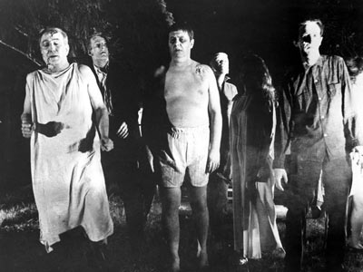
Zombies in George Romero's Night of the Living Dead.

Humans would not survive a zombie holocaust, or so current work suggests. The fact that reanimated corpses do not stop unless their brain is destroyed, coupled with an insatiable appetite for human flesh has proven to be a deadly combination.

However, the work produced by Munz et al. assumes that zombies and humans are well-mixed, meaning that zombies can be found everywhere there are humans. Realistically, the initial horde of zombies will be localised to areas containing dead humans, e.g. cemeteries and hospitals. In addition, by not initially separating humans and zombies, humans are not able to run and hide in order to try and preserve themselves. It is a well documented fact that zombies are deadly but slow moving. Due to their slow movements it is quite possible that, given sufficient warning, we would be able to outrun the zombies and produce a defensible blockade where humans could live safely. In order to do so, it would be useful to know just how long an infestation of zombies would take to reach our defences as this would give us an estimate of how long we would have to scavenge for supplies and weaponry in order that we may protect ourselves from these oncoming, undead predators.

If the reader currently does not have the time to understand the justification of the mathematics due to their impending doom, we would recommend skipping the maths and going straight to some useful results.

Random walks and diffusion

According to Munz et al, "the 'undead' move in small, irregular steps". This makes their individual movement a perfect model of a random walk. The "drunkard's" or random walk, as you would expect from the name, is a mathematical description of movement in which no direction is favoured. To give an intuitive idea of the motion, consider an inebriated person. They stagger backwards and forwards, lurching from one resting place to another. In figure 1 we illustrate this motion with zombies; since they will move around randomly bumping into one another they too will spread over the domain. Diffusion has two primary properties, it is random in nature, and movement is from regions of high densities to low densities.

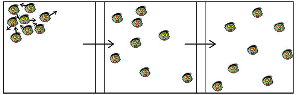
Figure 1: An example of two-dimensional diffusion. On the left an initial group of zombies is placed in the top-left corner, close together, their initial directions denoted by the black arrows. After a time their random motion will cause them to spread themselves out over the domain.

We could model the motion of each zombie individually but since their movement is random, unless we track them all exactly, their positions will not be certain. Probabilistic descriptions can be used but, due to the assumed large population of zombies, the computational power needed by such simulations would soon get out of hand, even when we are not running for our lives. Instead, we consider the case where there is initially a large number of zombies. This produces a continuous model of diffusion which is much easier to use as it needs less computational power and analytical solutions are available. However, what we have gained in simplicity we have lost in accuracy. Realistically the density of zombies in a region will be a discrete integer value, e.g. 1, 2, 3, . . . zombies/metres (assuming even a dismembered zombie counts as a whole one). Through this large number assumption we are forced to allow the density to take any value including non-integers. Thus, instead of the density being a discrete valued function, it has been "smoothed out" to form a continuous function.

A mathematical description of diffusion

In order to simplify the following mathematics we assume we are working in only one space dimension, denoted x, that is we're working on a line. This is not too restrictive as most results hold in two, or even three, dimensions. Realistically speaking, this assumption means that there is only one possible access point to our defences and thus the shortest distance between the group of zombies and us is a straight line.

If we let the density of zombies at a point $x$ and at a time $t$ be $Z(x, t)$ then the density has to satisfy the diffusion equation,

$\begin{equation} \frac{\partial Z}{\partial t} (x,t) = D \frac{\partial ^2 Z}{\partial x^2}(x,t) \end{equation}$

(1)

The term $\frac{\partial Z}{\partial t} (x,t)$ describes the rate of change of $Z$ over time at a point $x$ . This means if $\partial Z/\partial t$ is positive, then $Z$ is increasing at that point in time and space. This term allows us to consider how $Z(x,t)$ evolves over time.

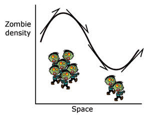
An example of how diffusion smoothes out peaks and troughs.

Figure 2. An example of how diffusion smooths out peaks and troughs.

The factor $D$ is a positive constant that controls the speed of movement. The units of $D$ are chosen to make the diffusion equation consistent since the units on each side of the equality must match. The term $\partial Z/\partial t$ has units of [density]/[time] and $\partial ^2 Z/\partial x^2$ has units of [density]/[space] $^2$ , thus $D$ must have units of the form [space] $^2$ /[time]. The units could be of the form of kilometres $^2$ /hour or nanometres $^2$ /second. However, for the equation to be most informative we choose scales which are relevant to a zombie invasion, thus we fix the units to be metres $^2$ /minute.

The term on the right-hand side of equation (1) is a little more complex than the left, but essentially it encapsulates the idea that the zombies are moving from high to low densities. This is illustrated with the help of figure 2. Initially, there are many more zombies on the left than the right. Just before the peak in density the arrow (which is the tangent to the curve, or $\partial Z/\partial x$ , at this point) is pointing upwards. This means that as $x$ increases, so does the zombie density, $Z$ . At this point

$\frac{\partial Z}{\partial x} = \mbox{rate of change of }Z\mbox{ as x increases }>0.$

Just after the peak the arrow is pointing down. Thus, at this point,

$\frac{\partial Z}{\partial x} = \mbox{rate of change of }Z\mbox{ as }x\mbox{ increases }<0.$

Hence, at the peak, $\partial Z/\partial x$ is decreasing as $x$ increases (because it moves from being positive to being negative). Since $\partial ^2 Z/\partial x^2$ is the rate of change of $\partial Z/ \partial x$ as $x$ increases and we have just deduced that $\partial Z/\partial x$ is decreasing at the peak,

$\frac{\partial ^2 Z}{\partial x^2} <0.$

From the diffusion equation we see that, at the peak,

$\frac{\partial Z}{\partial t} = D\frac{\partial ^2 Z}{\partial x^2} <0, $ this means that the peak of zombie density is decreasing over time. Similarly, $\partial Z/\partial x < 0$ just before the trough and $\partial Z/\partial x > 0$ after the trough, as shown in figure 2. Thus, at the trough, $\partial ^2Z/\partial x^2 > 0$, implying that the density of zombies is increasing. Overall we see that diffusion causes zombies to move from regions of high density to low density. $$

It is impossible to overstate the importance of equation (1). Wherever the movement of a modelled species can be considered random and directionless, the diffusion equation will be found. This means that by understanding the diffusion equation we are able to describe a host of different systems such as heat conduction through solids, gases (e.g. smells) spreading out through a room, proteins moving round the body, molecule transportation in chemical reactions, rainwater seeping through soil and predator-prey interaction, to name but a few of the great numbers of applications.

Solution to the diffusion equation

The diffusion equation gives us a mathematical description of zombie movement. By solving it we produce the function $Z(x, t)$ , the density of the zombies at each position x for all time $t \geq 0$ . However, we must add some additional information to the system before we can solve the problem uniquely.

Initially, we have a density of $Z_0$ zombies/metre. All of the zombies are assumed to start in the region $0 \leq x \leq 1$ . The implication of this is that all of the undead will originate from one place, say a cemetery or mortuary in a hospital.

The final assumption we make is that the zombies cannot move out of the region $0 \leq x \leq L$ . So there is a theoretical boundary at $x = 0$ that the population cannot cross; the zombies will simply bounce off this boundary and be reflected back into the domain. We place our defences at $x = L$ , thus creating another theoretical boundary here. Thus, at $x = 0$ and $x = L$ , the "flux of zombies" (the rate of change of zombies through the boundary) is zero. Various other boundary conditions are possible but for simplicity we chose zero flux conditions so that the boundaries may prevent the zombies from leaving the region but do not alter their population.

Mathematically, the flux of zombies through $x=0$ and $x=L$ is the spatial derivative at these points and since they are assumed to be zero then $\partial Z/\partial x = 0$ at $x = 0, L$ .

The system is then fully described as

$\frac{\partial Z}{\partial t}(x,t) = D\frac{\partial ^2 Z}{\partial x^2}(x,t),$

with the initial condition

$Z(x,0) = \left\{ \begin{array}{cc} Z_0 & \mbox{for }0\leq x \leq 1, \\ 0 & \mbox{for }x>1. \end{array}\right.$

and the zero flux boundary condition

$\frac{\partial Z}{\partial x} (0,t) = 0 = \frac{\partial Z}{\partial x} (L,t).$

This system, with these initial and boundary conditions, can be solved exactly and has the form

$Z(x,t) = \frac{Z_0}{L} + \sum _{n=1}^{\infty } \frac{2Z_0}{n\pi } \sin {\left( \frac{n\pi }{L}\right)} \cos {\left(\frac{n\pi }{L}x\right)} \exp {\left(-\left(\frac{n\pi }{L}\right)^2 Dt\right)}.$

The $\sin$ and $\cos$ functions are those that the reader may remember from their trigonometry courses. The exponential function, $\exp$ , is one of the fundamental operators of mathematics, but for now the only property that we are going to make use of is that if $a > 0$ then $\exp (-at) \rightarrow 0$ as $t \rightarrow \infty$ . Using this fact and the solution to our system, then as $t$ becomes large most of the right-hand side of the equation becomes very small, approximately zero. Hence, for large values of $t$ , we can approximate

$Z(x,t) \approx \frac{Z_0}{L}.$

This means that as time increases, zombies spread out evenly across the available space, with average density $Z_0/L$ everywhere.

In figure 3 we have plotted zombie density for a number of times; figure 3(a) shows the initial condition of a large density of zombies between $0 \leq x \leq 1$ . Figure 3(b) and figure 3(c) then illustrate how diffusion causes the initial peak to spread out filling the whole domain. Note that we rescaled the axes in figures 3(c) and 3(d) in order to show the solution more clearly. Figure 3(d) verifies our approximation when $t$ is large, since after 100 minutes the density of zombies has become uniform throughout the domain.

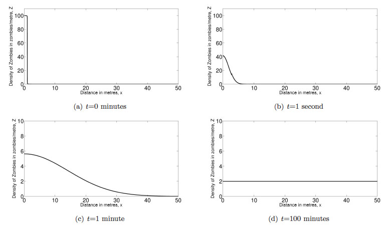
Figure 3: Evolution of a system of zombies over 100 minutes. The zombies are assumed to be confined within a domain of length 50 metres and have a diffusion coefficient of D = 100 metre²/minute.

Time of first interaction

Our solution gives the density of zombies at all places, $x$ , and for all time, $t$ . There are many questions we could answer with this solution, however, the most pressing question to any survivors is, "how long do we have before the first zombie arrives?" The mathematical formulation of this question is, "for what time, $t_ z$ , does $Z(L,t_ z) = 1$ ?". The time $t_ z$ is then the time taken (on average) for a zombie to have reached $x = L$ .

Unfortunately this does not have a solution that can be written down nicely. But thankfully there is a method (which we won’t describe here) which enables us to find this solution, approximated to any degree of accuracy we desire.

Using this technique we can now vary the distance and speed of the zombies to calculate the various interaction times. In figure 4 we plot the interaction time of an initial density of 100 zombies against a diffusion rate, ranging from $100m^2/min$ to $150m^2/min$ , which (from empirical evidence) is realistic for a slow shuffling motion, and for distances between 50 to 90 metres. 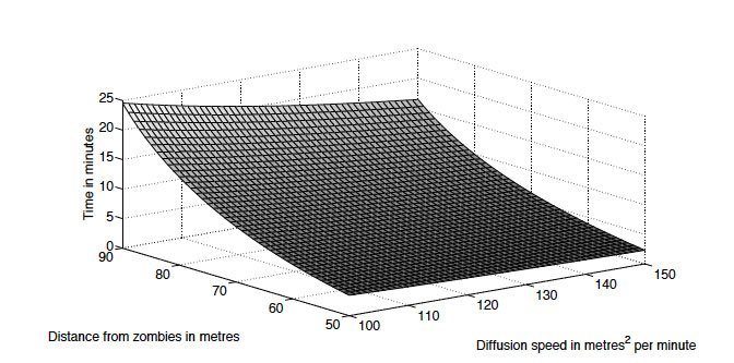Notice that for distances greater than $L = 100m$ , the average density of zombies is less than 1 zombie/metre and so there will be no solution, $t_ z$ , to $Z(L,t_ z) = 1$ since $Z(L,t) < 1$ for all $t \geq 0$ . In this situation the assumption that we have large number of zombies has failed thus causing the continuous model to be an inadequate description.

Figure 4: Time in minutes until the density of zombies reaches one for various rates of diffusion and distances.

Our approximate solution also answers another important question: should we delay the time of the inevitable first meeting by running further away, or by trying to slow the zombies down? As the above graph shows, increasing the distance between us and the zombies leads to a greater increase in the time of first interaction than a comparative decrease in their diffusion rate.

Since we want to delay interaction with the zombies for as long as possible, we see that it is much better to expend energy travelling away from the zombies than it is to try and slow them down since without some form of projectile weaponry or chainsaw, killing zombies is particularly difficult as they do not stop until their brain is destroyed.

It should be noted that the time derived here is a lower bound. In reality the zombies would be spreading out in two dimensions and would be distracted by obstacles and victims along the way, so the time taken for the zombies to reach us may be longer. The fact that this is a conservative estimate though will keep us safe since the authors would prefer to be long gone from a potential threat rather than chance a few more minutes of scavenging!

Conclusion

Our diffusion model can tell us how long we have before zombies arrive. But mathematics can also be used to find strategies for slowing the rate of zombie infection, and even to answer the questions of whether it is possible to survive at all. (For those of you behind a very solid barricade with time to spare, you might like to read about these techniques in the upcoming book Mathematical Modelling of Zombies.)

For those already holding off the undead hordes we can summarise our results. Running away is a more successful strategy than trying to slow the zombies down, thus fleeing for your life should be the first action of any human wishing to survive.

However, we cannot run forever; interaction with zombies is inevitable. Therefore mathematically the only way to survive is to erect a fortified society that can sustain the human population, whilst allowing us to remove zombies as they approach. However should the barricade fail or you are unable to even reach such a commune, your prospects are not good.

Our conclusion is grim, not because we want it to be so but because it is so. It had always been the authors' intention to try and save the human race. So to you, the reader, who may be the last survivor on Earth, we say run. Run as far away as you can get; an island would be a great choice. Only take the chance to fight if you are sure you can win and seek out survivors who will help you stay alive.

Good luck. You are going to need it.

About this article

This article has been adapted from a chapter of the book Mathematical Modelling of Zombies, which teaches mathematical modelling using the undead as an example. It is aimed at interested undergraduates or anyone who's interested in how mathematics can solve problems in the real world. The book comprises many contributors and has been edited by Robert Smith?.

About the authors

Thomas Woolley is Junior Research Fellow in Mathematics at St John's College, University of Oxford, and London Science Museum Fellow of Modern Mathematics. His research interests are in biological pattern formation and mechanisms of cell movement. He was Mathematics Advisor to the television show Dara O'Briain's School of Hard Sums, and awarded the Gibbs and IMA Junior Mathematics prizes for outstanding examination performances in Oxford.

Ruth Baker studied mathematics at the University of Oxford, before joining the Wolfson Centre for Mathematical Biology in Oxford for her doctoral studies. She was subsequently appointed to an RCUK Fellowship in Mathematical Biology, and more recently to a University Lectureship, both also in the Wolfson Centre for Mathematical Biology. Her research interests include mathematical modelling of aspects of developmental biology, including self-organisation, cell motility and domain growth. Her knowledge of zombie behaviour has increased exponentially during this project.

Eamonn Gaffney studied mathematics at the University of Cambridge, prior to a PhD in theoretical high energy physics and a Wellcome Trust Post-Doctoral Fellowship at the Centre for Mathematical Biology Oxford. After a faculty position at the School of Mathematics, University of Birmingham, he returned to a University Lectureship at Oxford and the Wolfson Centre for Mathematical Biology in 2006. His research interests include microbiological continuum mechanics, biological self-organisation and cell motility, signalling and interactions.

Philip Maini gained his DPhil in mathematical biology under the supervision of Jim Murray. He is Professor of Mathematical Biology and Director of the Wolfson Centre for Mathematical Biology, Oxford. His research interests include the application of mathematical modelling in areas in developmental biology, wound healing and cancerous tumour growth.

Plus.Maths.org