
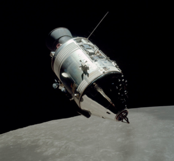
Hide and seek: Tracking the Apollo spacecraft was a challenge for NASA scientists.
When NASA first decided to put a man on the Moon, they had a problem. Actually, they had several problems. It was the spring of 1960, and not only had they had never sent a man into space, the Soviet Union had recently won the race to put a satellite in orbit. Then there were the technical issues: the nuts and bolts of how to transport three men 238,900 miles from a launch site in Florida to the Moon – and back again – all before the Soviets beat them to it.
One of the biggest stumbling blocks was estimating the spacecraft's trajectory: how could NASA send astronauts to the Moon if they didn't know where they were? Researchers at NASA's Dynamics Analysis Branch in California had already been working on the problem for several months, with limited success. Fortunately for the Apollo programme that was about to change.
Randomness and errors
Working out the trajectories had proven difficult for the researchers because they were really trying to solve two problems at once. The first was that spacecraft don't accelerate and move smoothly in real life, as they might in a physics textbook. They are subject to variable effects like lunar gravity, which are often unknown. This randomness meant that even if the scientists could have observed the craft's exact position, the trajectory wouldn't follow a neat, predictable path.
But that was their second problem: they couldn't observe its exact position. Although onboard sensors included a sextant, which calculated the angle of the Earth and Moon relative to the spacecraft, and gyroscopes, it wasn't clear how this data – which inevitably contained measurement errors – could be accurately translated back into position and velocity.
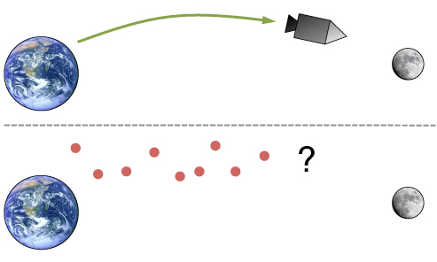
Top: In a perfect world the spacecraft would have a simple, textbook trajectory. Bottom: In reality its movement is subject to randomness, and so are the measurements used to estimate its (unknown) position.
Stanley Schmidt, the engineer who led the Dynamics Analysis Branch, had initially hoped to use ideas developed for long-range missiles, another product of the Cold War rivalry with the Soviet Union. However, missile navigation systems took measurements almost continuously, whereas during a busy mission the Apollo craft would only be able to take them at irregular intervals. Schmidt and his colleagues soon realised that existing methods wouldn't be able to give them accurate enough estimates: they needed to find a new approach.
What happened next was an incredible stroke of good luck. In the autumn of 1960, an old acquaintance of Schmidt's – who had no idea about the work the NASA scientists were doing – called to arrange a visit. Rudolph Kalman was a mathematician based in Baltimore, and he wanted to come and discuss his latest research.
The Kalman filter
Kalman specialised in electrical engineering and had recently found a way of converting a series of unreliable measurements into an estimate for what was really going on. His mathematical results had been met with scepticism, though, and Kalman had yet to find a way to turn his theory into a practical solution.
Schmidt didn't need convincing. After hearing Kalman's presentation, he distributed copies of the method to the NASA engineers and worked with Kalman to develop a way to apply it to their problem. By early 1961 they had their solution.
Kalman's technique was called a filter and worked in two steps. The first used Newtonian physics to make a prediction about the current state of the system (in NASA's case the location of the spacecraft) and the level of uncertainly due to possible random effects. The second step then used a weighted average to combine the most recently observed measurement, which inevitably had some degree of error, with this prediction.
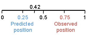
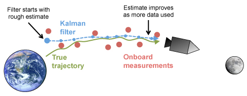
The Kalman filter compares predictions using Newton's Laws with onboard measurements to generate a better estimate of the spacecraft's true position.
As well as producing accurate estimates, the Kalman filter could run in real time: all it needed to generate an estimate were the previous prediction and current onboard measurement. Because any calculations would have to be done on the Apollo's primitive on-board computer this simplicity made the filter incredibly valuable. In fact, it would eventually be used on all six Moon landings, as well as finding its way into the navigation systems of nuclear submarines, aircraft and the International Space Station.
From trajectories to transmission
Decades after the Moon landings questions still remain about how best to estimate hidden information, and it's not just engineers asking them. Disease researchers have long wondered how to understand the true spread of an infection (which they can't see) using hospital case reports (which they can). In some ways it's not that different from the problem NASA had. Even if researchers try and make predictions by assuming a disease transmits in a certain way, its spread will still be affected by randomness. And it's unlikely the proportion of infected people who go and see a doctor will remain constant, which means any measurement method – for example, assuming hospital reports represent a certain fraction of total infections – is also subject to error.
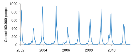
Reported influenza cases in France. The true level of infection may be different.
Unfortunately NASA's solution isn't much help when it comes to epidemics. The Kalman filter only works for specific types of problem in which we can write down an equation for what the system should be doing in theory. That might be the case for spacecraft trajectories and other physics-based puzzles, but it's less so when dealing with complex biological systems. Instead, we are forced to simulate lots of outbreaks, each influenced by random effects, in the hope of discovering which ones line up with the hospital data.
Of course running a huge number of simulations requires a lot of effort. Ideally we want a way of keeping predictions that agree with the case reports over time, and throwing out the ones that don't. This can be done with a method known as a particle filter. Whereas the Kalman filter makes a single prediction at each point in time, then adjusts it using the observed data, a particle filter uses simulations to make a large number of predictions (the particles) at each point in time. These particles – which are all different because of the randomness in the system – are then weighted based on how likely they are to produce the observed data, and the "lighter" particles pruned away (the filter). In essence, it's a process of natural selection: over time, the best predictions survive, and the weaker ones fall by the wayside.
Making the right predictions
Particle filters rely on computer simulations which assume that the disease transmits in a particular way. In other words, we are assuming that a specific mathematical model is a good reflection of reality. The reason why one model can give rise to lots of different simulations is that the model incorporates randomness, so each time we run it you get a different outcome. But what if – as is often the case – we don't know how an infection actually spreads? Cholera is a good example: outbreaks in India and Bangladesh have puzzled researchers for years.
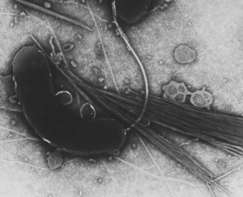
Cholera bacteria are responsible for thousands of deaths each year.
Most cholera infections don't result in symptoms, which means it is very difficult to know where new infections come from, or how many there really are. As a result there are many unanswered questions about why cholera outbreaks happen. Do infections come from mainly from other people or local water sources? How quickly do previously infected people lose immunity to the disease? What effect do the symptomless infections have on the spread of cholera bacteria?
There are several possible answers to such questions and therefore several different models we could use to simulate outbreaks. We really need a way to compare the various models and this is where particle filters can help. By finding the best prediction each model is capable of making (specifically, the prediction that has the highest likelihood of generating the observed patterns) we can see which model comes out top.
When researchers compared different models for cholera they found that the real data could be best reproduced with a large number of symptomless individuals, immunity that fades quickly, and infection arriving both from other people and the local environment. In fact, they did one better than that. By adapting the particle filter, they found a way to estimate values such as the duration of immunity at the same time as selecting the best prediction. According to the model, the period of immunity was around 9 weeks, far lower than previously thought.
Particle filter techniques are useful for other diseases too: recent work has looked at how population structure affects the spread of measles and why influenza pandemics occur as waves of infection. The methods allow researchers to take a number of different theories about the hidden causes of epidemics and test them against the limited information they do have. As such, they are proving to be an increasingly important public health tool.
Modern solutions to an age-old problem
Years after the Apollo program finished, Stanley Schmidt and one of his colleagues produced a report documenting their work on the trajectory predictions. As expected they had plenty of praise for the Kalman filter. "The broad application of the filter to seemingly unlikely problems suggests that we have only scratched the surface when it comes to possible applications," they wrote, "and that we will likely be amazed at the applications to which this filter will be put in the years to come."
It turned out to be a shrewd prediction. Disease researchers now employ filters to work out what causes outbreaks. Atmospheric scientists use them to make sense of weather patterns. Economists apply the methods to financial data. The techniques may have begun as a way to guide three men to the Moon, but they have since evolved into a valuable set of tools for tackling problems back here on Earth.
About the author
Adam Kucharski is a PhD student in applied mathematics at the University of Cambridge. His research covers the dynamics of infectious diseases, focusing on influenza in particular. He has recently won the Wellcome Trust science writing prize.