

The Mandelbrot set. Image Wolfgang Beyer.
If you're bored with your holiday snaps, then why not turn them into fractals? A new result by US mathematicians shows that you can turn any reasonable 2D shape into a fractal, and the fractals involved are very special too. They are intimately related to the famous Mandelbrot set.
The new result, which was proved by Kathryn A. Lindsey and the late William P. Thurston, works for any shape whose outline is made up of a finite collection of simple closed curves. These are continuous loops in the plane that don't intersect themselves. The fractals involved come from seeing how points in the plane are moved around by a particular class of mathematical function.
To understand how this works, think about the quadratic function $$f(x)=x^2.$$ When you plug $x=0$ into the function, the result, $$f(0)=0^2=0,$$ is again 0, so 0 is what's called a \emph{fixed point}. The same happens with $x=1, $ as $$f(1)=1^2=1.$$ Other values of $x$, however, are more interesting. Take $x=2$ for example. We get $$f(2)=2^2=4.$$ If you now apply the function again using 4 as your new value for $x$ you get: $$f(4)=4^2=16.$$ Using 16 as the new value for $x$ you get $$f(16) = 16^2=256.$$ You can see what happens if you repeat this process, always using the result of your last calculation as the new value for $x.$ The numbers you get become bigger and bigger, in fact you can make arbitrarily large numbers just by repeating this procedure. The sequence of numbers you get in this way, starting with the number 2, is called the \emph{orbit} of 2 under the function $f$, and we say that the orbit of 2 \emph{escapes to infinity}. In fact, for this particular function the orbit of any number that is bigger than 1 or smaller than -1 escapes to infinity. But what happens for numbers that lie between -1 and 1, that is, for $-1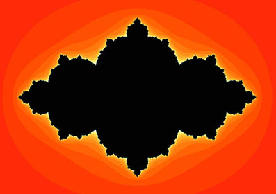
The black area is the filled Julia set of a quadratic polynomial. Its outline is the Julia set.
But what does all of this have to do with shapes in the plane? In the examples above the polynomial functions were applied to the points that lie on the number line. But there's a way of turning them into functions that can be applied to points in the plane, so that the function sends every individual point $(x,y)$ to some other point $(z,w)$ in the plane. To do this you need to use \emph{complex numbers}.(See the article Unveiling the Mandelbrot set for details.)
Just as before with the number line, a function f now gives a partition of the plane into points with escaping and points with trapped orbits. The set of points with trapped orbits is called the filled Julia set of the function (after the French mathematician Gaston Julia). And the boundary of the filled Julia set, its outline, is called simply the Julia set. Generally Julia sets of polynomials are fractals: shapes of infinite complexity. Their crinkly outline remains just as crinkly, no matter how closely you zoom in on them. (See this article for more on fractals.)
The new result says that any simple closed curve in the plane can be approximated by the Julia set of a polynomial — you can match the curve by the Julia set — and that such an approximation can be made as precise as you like. If you're trying to approximate a whole collection of simple closed curves, you may need to use functions that are slightly more complicated. They are called rational functions and are what you get from dividing one polynomial by another. The collection of curves can then be approximated by parts of the Julia sets of these functions.

A Julia set in the shape of a cat. To see its crinkliness, look at this larger version. Image: Kathryn Lindsey and William Thurston.
And what's the connection to the Mandelbrot set? It turns out that the points on the plane can be used to label quadratic polynomials: every single quadratic polynomial can be associated to exactly one point in the plane (see Unveiling the Mandelbrot set for details). The points that belong to the Mandelbrot set, coloured black in the picture of the Mandelbrot set above, correspond to quadratic polynomials whose Julia sets consist of just one component, rather than a collection of separate chunks. The Mandelbrot set is itself a fractal and it's pretty universal. It doesn't only come up in connection with quadratic polynomials, but also in connection with many other classes of functions.
A preprint paper of the new result has been published on arxiv.org. Not the easiest way of spicing up your photos perhaps, but one that will delight mathematicians.