This article is part of the Researching the unknown project, a collaboration with researchers from Queen Mary University of London, bringing you the latest research on the forefront of physics. Click here to read more articles from the project.

You know you are on to something when complicated things suddenly become easy. It's what happened ten years ago, when three physicists from Queen Mary University of London, decided to dabble in an area of physics they didn't know much about. Within a few months they had developed a ground breaking new technique, combining new ideas with methods that came from a dusty old textbook of outdated physics. At the heart of their success lies a new way of drawing pictures.

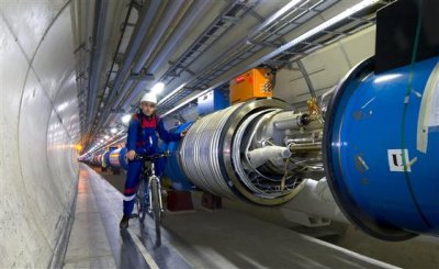
The Large Hadron Collider. It's in particle accelerators like this one that unknown particles like the Higgs boson are produced. Image © CERN.

The challenge they took on concerned a surprising problem of particle physics. There is a theory, the standard model of particle physics, that describes the fundamental particles of nature and their interactions through all but one of the fundamental forces (gravity being the exception). The theory has been successful in many ways, but it is hard to make even basic predictions, such as what you expect to happen when two particles collide, at least not exactly. The calculations are so lengthy and complex, they beat even the fastest supercomputer. Without such predictions, however, you can't test your theory against reality and you will find it hard to spot whether an experiment has produced something new.

In practice physicists make do with approximate answers, and in many cases these are good enough. For example, last year they confirmed the existence of the celebrated Higgs boson, detected in the Large Hadron Collider (LHC) at CERN, beyond reasonable doubt. But as technology advances, more accurate calculations will become necessary. And anyway, there is something worrying about a theory you can't actually calculate with. Andreas Brandhuber, Bill Spence and Gabriele Travaglini's work is an encouraging step in the right direction: it can transform weeks' worth of computer calculations into something that could be done on a single page in an hour.

Let me count the loops...

The idea behind particle accelerators, like the LHC, is that interesting things happen when particles collide. It's not a new idea. In 1909 Ernest Rutherford and his colleagues fired alpha particles into tin foil and found that some of them scattered off it in a way that the known laws of physics didn't allow. Rutherford declared this to be "quite the most incredible event that ever happened to me in my life," and went on to develop a new model of the atom that explained the observations.

Figure 1: This image is a Feynman diagram of electron-electron scattering. The solid lines represent the particles' paths through space time and the wiggly line denotes the propagation of a virtual photon, emitted at x₅ and absorbed at x₆.

The LHC collides highly energetic protons, and it is in these collisions that new particles such as the Higgs bosons are produced. To predict what they expect to happen in the collider, physicists need to calculate scattering amplitudes: essentially these tell you the probabilities that certain new particles are produced when two particles smash into each other. It's these scattering amplitudes that pose the computational challenge.

The problem is that a collision involves more than just incoming and outgoing particles. For a fleeting instant, any number of unobservable virtual particles might pop into existence, interact, and then disappear again. One, two, three, or any number of virtual particles could be produced and interact in different ways. In principle all possible configurations need to be taken into account when calculating the scattering amplitude. The resulting maths is horrendous. When the physicist Hans Euler made some pioneering calculations in 1936, an interaction involving just one pair of virtual particles required over six pages of maths. (See this article for more on virtual particles.)

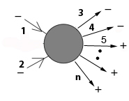
Figure 2: This image shows all the ways in which two electrons can scatter by exchanging two photons. Image adapted from a figure in Richard Feynman's article Space-time approach to quantum electrodynamics. Copyright (2013) by The American Physical Society.

In the 1940s the Nobel Prize winning physicist Richard Feynman caused a revolution in its own right. He came up with stick-figure-like diagrams which exactly capture the calculations, but also chime with intuition (see figure 1). Feynman's invention was pure genius. Physicists could now keep track of their sums pictorially, using a dictionary that precisely translates a diagram into mathematical expressions. The diagrams look as if they trace the paths of colliding particles, but they don't: they are unphysical pictures, drawn in spacetime rather than just space, which represent probabilities rather than real particle paths. Some Feynman diagrams contain little circular paths — loops. The more virtual particles are involved the more loops there are, and the further away the interaction is from classical physics in which these strange ghost-like things have no part. (See this article for more on Feynman diagrams).

Feynman diagrams have been a massive help for generations of physicists, but there is only so much they can do. There's a Feynman diagram for each type of particle interaction, defined by how many virtual particles are involved and how (see figure 2 for an example). Calculating a scattering amplitude exactly would mean chugging through an infinite number of Feynman diagrams. "That is the practical bottleneck of these Feynman rules," says Travaglini. "It just became too complicated to produce theoretical predictions which had enough precision to confront data." In practice physicists have been ignoring almost all of these possibilities and mostly considered diagrams that have no loops at all, called trees, or those that have just one loop. It's possible to do this because higher loop diagrams contribute progressively less to the overall calculation.

Know MHV, know physics

The MHV amplitude

Suppose you have two gluons coming into an interaction and n-2 coming out, so there's a total of n of them. The helicity of a gluon can be either + or -. Suppose the two incoming ones have negative helicity. If all outcoming gluons, or all but one outcoming gluon, have positive helicity, then the tree-level amplitude is zero. If exactly two outcoming ones have negative helicity then that's the MHV amplitude.

Its tree-level formula, first written down by Michelangelo Mangano, Stephen Parke and Zhan Xu, is surprisingly simple. We'll display it here without explanation so you can see how simple it is:

(Something similar works if more than two gluons come into the interaction and if you swap the helicities.)

If three outcoming gluons have negative helicity you get next-to-MHV, with four you get next-to-next-to-MHV and so on. No nice formulae were known for these amplitudes, but they correspond to collections of intersecting lines in twistor space and can be computed using MHV diagrams.

In the 1980s the physicists Stephen Parke and Tomasz Taylor encountered a mystery. They considered interactions involving particles called gluons which live inside protons. "Protons are not fundamental particles themselves," explains Brandhuber. "They are garbage bags, made up of bound states of quarks and gluons." When protons collide, quarks and gluons are liberated and can themselves collide. Understanding gluon and quark scattering is especially important, as they provide the background noise against which anything new, such as a Higgs boson, might show up.

Calculating gluon scattering amplitudes is complicated: an interaction that involves 10 gluons (as incoming and outgoing particles) comes with 10,525,900 Feynman diagrams, and that's only at tree-level, ignoring the loops. If you could calculate one diagram per second the calculation would take you 121 days! So Parke and Taylor were surprised to find that for a particular type of gluon interaction the scattering amplitudes at tree level seemed to be captured by a very simple formula. "So we had this quantity which was extremely simple, but the only way to go there was through enormous [calculations]," says Travaglini. "That was completely mysterious." The amplitudes in question are called maximally helicity violating (MHV) amplitudes — we will see how their mystery was solved on the next page.

About this article

Marianne Freiberger, Editor of Plus, interviewed Andreas Brandhuber and Gabriele Travaglini in London in November 2013.

Andreas Brandhuber.

Gabriele Travaglini.