Add new comment

Polar power

Cartesian coordinates.

Most of us are familiar with the Cartesian coordinate system which assigns to each point $p$ in the plane two coordinates $(x_0,y_0)$ . To find $p$ you start at the point $(0,0)$ and walk a distance $x_0$ along the horizontal axis and a distance $y_0$ along the vertical axis (see image on the right).

But there’s another way of locating points on the plane, which is very nice too. To each point $p$ assign the pair of numbers $(r, \theta )$ , where $r$ is the distance from $(0,0)$ to $p$ along a straight radial line, and $\theta$ is the angle formed by that radial line and the positive $x$ -axis, measured anti-clockwise from the $x$ -axis to the line. These new coordinates are called polar coordinates, because you treat the crossing point of the axes as a pole from which everything radiates out.

In the image below, click on the point and drag it around to see how its polar coordinates $(r, \theta )$ change (degrees are measured in radians).

How do you express simple shapes in polar coordinates? As you can see from the interactivity above, a ray that starts at the point $(0,0)$ is given by a particular value of the angle $\theta .$ For example, the positive $y$ -axis is described by the equation

$\theta =\pi /2 = 1.5707...$

and the ray that halves the angle between the positive $x$ and $y$ -axes is given by the equation

$\theta =\pi /4 =0.7853... .$

Generally, the equation

$\theta = \theta _0$

describes the ray that starts at $(0,0)$ and makes an angle $\theta _0$ with the positive $x$ -axis.

What about circles? A circle centred on $(0,0)$ of radius $r_0$ consists of all points that lie at distance $r_0$ from $(0,0)$ . So we can describe the circle in polar coordinates using the equation

$r = r_0.$

This expression is a lot simpler than the equation of a circle in Cartesian coordinates, which is

$x^2+y^2 = r_0^2.$

The polar equations describing lines that don't pass through the point (0,0) and circles that are not centred on (0,0) are more complicated than their Cartesian versions (see here). But there are shapes whose description using polar coordinates are a lot simpler than their Cartesian counterparts. Here are three of our favourite examples.

Archimedean spirals

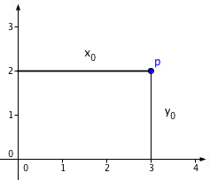
Let’s look at all the points whose polar coordinates $(r, \theta )$ satisfy the equation

$r=\theta ,$

in other words, we are looking at points with polar coordinates $(\theta , \theta ).$ Where are they?

The animation below shows the ray corresponding to the angle $\theta$ as $\theta$ ranges from 0 to $2\pi$ . The point $p$ marked on the ray is the one with coordinates $(\theta , \theta ).$ As $\theta$ increases the point moves further away from $(0,0).$ (Click on the play icon in the bottom left hand corner or use the slider to vary $\theta$ .)

We have the beginning of a spiral!

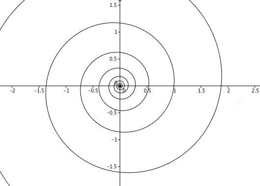
But why stop at $2\pi$ ? You could keep turning the radial line by more than one full turn, through one-and-a-half turns ( $3\pi$ ), two turns ( $4\pi$ ), and so on, round and round. Then, as $\theta$ goes through another full turn from $2\pi$ to $4\pi$ , the distance to $(0,0)$ of the point $p$ with coordinates $(\theta , \theta )$ increases further, from $2\pi$ to $4\pi$ . Letting $\theta$ run from $4\pi$ to $6\pi$ gives us another full turn with points moving out even further. The animation below shows the spiral you get from letting $\theta$ vary from 0 to $20\pi .$

Letting $\theta$ increase all the way to infinity gives a spiral that loops around $(0,0)$ an infinite number of times:

This beautiful shape is called an Archimedean spiral, named after the great Greek mathematician Archimedes who discovered it in the third century BC. As you can see from the picture, the loops of the spiral are evenly spaced: if you draw a radial line from $(0,0)$ , then the distance between two successive intersection points with the spiral is always $2\pi$ .

There are other Archimedean spirals too, all characterised by the fact that a radial line intersects the spiral at equal intervals. They can be characterised by the equation

$r=a\theta$

for $a$ a positive real number. By playing around with different values for $a$ you can convince yourself that $a$ controls how tightly the spiral is wound up, and therefore the distance between successive intersection points along a radial line. For a psychedelic experience (or to give yourself a headache) try the animation below with shows Archimedean spirals with $a$ varying from 5 down to 0.

If you prefer a physical interpretation, an Archimedean spiral is what you get when you trace the path of a point that moves out from the centre at constant speed along a line that rotates with constant angular velocity.

Logarithmic spirals

Now let’s look at all points whose polar coordinates $(r, \theta )$ satisfy the equation

$r = e^{\theta /10},$

where $e$ is the base of the natural logarithm, $e = 2.71828...$ .

When $\theta =0$ , we get

$r = e^{0} = 1,$

So our shape contains the point with polar coordinates $(1,0)$ (whose Cartesian coordinates happen to also be $(1,0)$ ). The animation below shows the radial line corresponding to the angle $\theta$ as it varies from $0$ to $2\pi .$ The point $p$ with coordinates $(e^{\theta /10},\theta )$ is marked too. Again we see the beginning of a spiral but this time a different one.

Again we can let $\theta$ range beyond $2\pi$ , through $4\pi$ , $6\pi$ and so on, giving a spiral that winds around any number of times. This time, however, the loops of the spiral are not evenly spaced.

This is an example of a logarithmic spiral. It carries this name because instead of writing

$r = e^{\theta }$

you could write

$\theta = \ln {r},$

where $\ln$ is the natural logarithm to base $e$ .

(There is also a more general form of the logarithmic spiral, given by the equation

$r = ae^{b\theta },$

where $a$ and $b$ are positive real constants. )

But there is another trick we can play here: we can allow the angle $\theta$ to become negative! To find a point whose second polar coordinate is negative you measure the angle from the positive $x$ -axis in the other direction: clockwise. For example, a point with polar coordinates $(r,-\pi /2)$ lies on the negative part of the $y$ -axis.

What does this mean for our logarithmic spiral? As $\theta$ moves from $0$ towards negative infinity, the radial line given by $\theta$ turns clockwise through one, two, three, and any number of turns. The points $p$ with coordinates

$p = (e^{\theta /5}, \theta )$

lie on that radial line. But now as $\theta$ decreases toward negative infinity, the points move inward, towards $(0,0).$ This is because

$e^{x} = 1/e^{-x},$

so if $x$ is very negative, then $e^{-x}$ is a very large number, so $1/e^{-x}$ is positive and very close to 0.

The animation below shows the point $p$ as $\theta$ varies from $0$ down to $-20\pi .$

Letting $\theta$ range all the way from negative to positive infinity creates a spiral that is infinite in both directions, it has no beginning and no end.

A full logarithmic spiral.

But hang on a second. This picture looks pretty much the same as the one you get from the animation above it, even though the x and y-axes here cover a much smaller range, as you can see from the labels! This illustrates a very interesting property of logarithmic spirals. If you zoom in or out of a picture of a logarithmic spiral, the picture you see looks exactly as it did before you zoomed. That feature is called self-similarity. It may be the reason why logarithmic spirals are so common in nature. You can see them in the turns of a snail shell, in many plants and even in the arms of spiral galaxies. The 17th century mathematician Jacob Bernoulli was so fascinated by this beautiful shape, he called it the "spiral mirabilis" (miraculous spiral) and asked for it to be engraved on his tomb stone, along with the sentence "Although changed, I shall arise the same." Unfortunately the engravers got it wrong and he ended up with an Archimedean spiral on his grave instead.

Polar roses

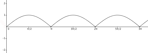
For our final shape, or rather family of shapes, let’s start by considering the equation

$r = |\sin {\theta }|$

(The || symbol stands for the absolute value, so we are only considering positive numbers for $r$ .)

To see what is going on here, let’s first recall the shape of the sine function, plotting $\theta$ on the horizontal axis against $\sin {\theta }$ on the vertical one: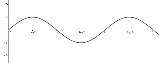

Applying the absolute value means that the parts of the wave that are below the horizontal axis (for which $\sin {\theta }$ is negative) are flipped to lie above it:

You can see that as $\theta$ moves from $0$ to $\pi$ , the value of $|\sin {\theta }|$ moves from 0 to a maximum of 1 (at $\theta = \pi /2$ ) and back down to 0.

Now let’s go back to our polar coordinates. As $\theta$ ranges from $0$ to $\pi$ , the distance to $(0,0)$ of our points

$p = (|\sin {\theta }|, \theta )$ ranges from 0 (at $\theta = 0$) up to 1 (at $\theta = \pi /2$) and back to $0$ (at $\theta = \pi $.) This creates a little loop in the upper half plane. Then as $\theta $ moves from $\pi $ to $2\pi $ the distance $|\sin {\theta }|$ varies in exactly the same way. This creates a little loop in the lower half plane. $$

Now let’s up the stakes and consider the equation

$r = |\sin {2\theta }|.$

The new factor of 2 means that the two loops that previously appeared for $\theta$ ranging from $0$ to $2\pi$ now appear for $\theta$ only ranging only from $0$ to $\pi$ . This means that both loops occur in the upper half plane and also become a little squashed. As $\theta$ moves on from $\pi$ to $2\pi$ , the value of $2\theta$ ranges from $2\pi$ to $4\pi .$ Since the sine function is periodic (it has the same value for $\theta +2\pi$ as it does for $\theta$ ) a mirror image of our pair of loops now also appears in the lower half plane:

We have a flower with four petals!

What happens if we consider the equation

$r = |\sin {k\theta }|,$

where $k$ is any positive whole number? You’ve guessed it! You get a flower with $2k$ petals — below we show you the results for $k=3$ and $k=10$ .. It’s amazing what polar coordinates can do!

About the author

Marianne Freiberger is Editor of Plus.

Polar power

Archimedean spirals

Logarithmic spirals

Polar roses

About the author

Filtered HTML