

A key result of last year's UN climate change conference in Paris is that we now have a new international deal to curb climate change. However, it seems primarily focused on reducing greenhouse gas emissions to limit global warming. A significant step forward, no doubt, but it does not address the more difficult, and perhaps also more relevant question of how to deal with the inevitable consequences of climate change. Are we able at all to predict what those consequences will be? And, more importantly, will we be able to do something to reduce, or even prevent, some of these consequences? When it comes to biodiversity and the distribution of species, some researchers believe this is indeed possible.
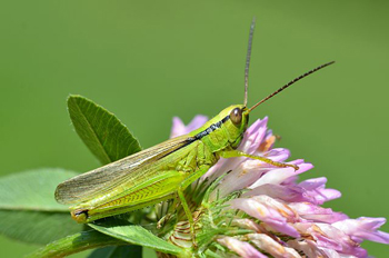
Mecostethus parapleurus is benefitting from mathematical modelling. Image: Giles San Martin, CC BY-SA 2.0.
.jpg)
The Spatial Ecology Group of Antoine Guisan at the University of Lausanne, Switzerland, studies species distributions, invasion patterns, and biodiversity using sophisticated mathematical modelling techniques. They are particularly interested in how climate change affects the current and future distribution and diversity of various (groups of) species.
Their main study area covers about 700km2 in the western part of the Swiss Alps. For this region, they have extensive data on the occurrences and absences of many plant species (such as Ranunculus platanifolius, a type of buttercup) and several insect species (such as Mecostethus parapleurus, a type of grasshopper), as well as fungi and bacteria. This data was collected by careful sampling and identification over many years of field work campaigns. The field data was then combined with detailed topographic information (such as elevation and slope), climatic data (such as average temperature and rainfall), and also soil and land use type, for the entire study area.
Next, the group used state-of-the-art mathematical modelling techniques to infer under what particular combination of environmental conditions each species thrives. For example, some plant species will grow only under relatively wet conditions in valleys with lots of sunshine, whereas other species are most happy under dry and cold conditions at high altitude. And some of the modelling techniques used to make these inferences have names that sound just as exotic as the actual species under study, including methods such as Generalised Boosted Regression Models, Artificial Neural Networks, or Flexible Discriminant Analysis. Despite the complicated names, the idea behind modelling the distribution of species is quite simple — we'll have a look at it below.

Ranunculus platanifolius, a type of buttercup, is also being studied by the Spatial Ecology Group. Image: Enrico Blasutto, CC BY-SA 3.0.
Finally, the inferred environmental preferences are used to predict how the distribution and diversity of species will change with particular changes in climate, for example an increase in average temperature. As one would expect, the models clearly show that in such a scenario some species will move away from the valleys and up the mountain slopes (in search of cooler temperatures), whereas other species currently already living at the highest altitudes will go extinct, as they have nowhere to escape to. More importantly though, the models can also predict with a high degree of accuracy what the actual magnitude and extent of these species distribution shifts or extinctions will be.
Perhaps more surprisingly, the models predict that significant extinctions might not occur until several decades from now. However, and alarmingly so, the models also indicate that the only way to prevent, or at least reduce, such future extinctions is by taking action now. If we want to maintain a certain level of biodiversity, we will have to start designing and implementing preservation policies today, such as the creation of protected wildlife areas and migration corridors, and a change to more sustainable farming and land development practices.
Given the large amounts of detailed data involved, and the sophisticated mathematical modeling techniques used, these studies require enormous computing resources. As a computer scientist I have worked with Guisan and his group to provide some of this required computational support. For example, I helped with getting their models to run on a large computer cluster, enabling them to do in several days what would otherwise have taken many months. Also, together with (then) graduate student Robin Engler, we implemented a species migration simulation model, which is now available as a free and open-source software package. And together with postdoctoral researcher Olivier Brönnimann, we came up with a mathematical method to reconstruct the most likely routes invasive plant species have taken in their dispersal.
The impact
The work of the Spatial Ecology Group has received increasing attention recently, and is also starting to have a real impact on environmental policy design and implementation. One of their success stories is the re-introduction of the otter in certain areas in Switzerland, largely based on modelling work done by (then) graduate student Carmen Cianfrani. Furthermore, the group has an important publication about their work in the high-profile journal Science, and Guisan has recently been ranked by Thomson-Reuters as one of the most cited scientists in the category Ecology/Environment. In short, these researchers certainly have something to say about the expected consequences of climate change, and how to possibly deal with some of them.
However, what if the projected future climate scenarios that are used in these models are wrong? For example, the overall warming trend seemed to have levelled off during the first decade of the new millennium. Most climatologists, though, believe that this is only a temporary deviation from the general trend, and that in the long run global temperatures will continue to rise. After all, both 2014 and 2015 were some of the warmest years on record, globally.
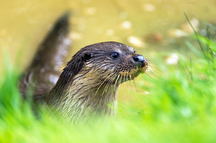
The otter has been reintroduced in certain areas in Switzerland, largely as a result of modelling work.
But even if the future climate projections are, somehow, incorrect, it would not invalidate the group's mathematical modelling techniques. The models would simply have to be run again, but with corrected future climate scenarios. After all, given a reliable set of input values, the species distribution models have already shown their predictive power and validity in many actual case studies.
Although most of the results mentioned above are specific to the group's main study area in the Swiss Alps, the methods are of course more general. Indeed, the same mathematical modelling techniques have been applied to other regions and species as well, such as arctic fish, and even on a world-wide scale. And in most cases the predictions are not any more optimistic, also calling for action and preservation right now, before it is too late.
So, instead of simply shrugging our shoulders and ignoring the inevitable, let's use the latest mathematical modelling techniques available to deal with the consequences of climate change in a responsible way. After all, this is not just about some plant species possibly going extinct. In the long run, the very existence of our own species could be at stake.
How to model the distribution of species
The mathematics behind species distribution models (SDMs) is conceptually easy. However, in practice SDMs are often cumbersome to use due to the large amounts of data and the intricate details of the specific mathematical models involved.
The figure below illustrates the basic idea. The gray shape at the top-left shows an outline of the original study area in the Swiss Alps. This area is divided into equally-sized squares, for example 1km by 1km each, or 25m by 25m for a more detailed resolution. Each square is identified by its coordinates (latitude & longitude).
Now, for a particular species it is known from the field work observations in which locations (squares) this species is present (the red dots in the study area). Let's say there are 100 such known "presences". Next, an equal (or at least similar) number of "absences" is selected by randomly picking locations from within the study area where there is no presence (the black crosses). Together, this defines an array (technically a vector) of 200 zeroes and ones: a zero denotes the absence of the species in the corresponding location and a one denotes its presence. We'll call this vector $y$.
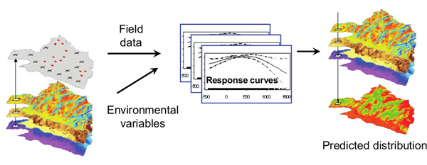
The information on the presence and absences of a species in an area (gray layer on the left) is correlated with environmental information for the area (coloured layers on the left) by a mathematical function f. The function can then be used to predict where the species will be present or absent when the environmental information changes. This then gives a predicted distribution corresponding to a particular environmental scenario (bottom layer on the right). Figure: Antoine Guisan, University of Lausanne, Switzerland.
In practice, this function estimation is often repeated many times with different sets of random absences, and using different (sometimes quite complicated) mathematical models and estimation techniques. This way, it is attempted to find the function that best fits the data. The accuracy of the different function estimations is evaluated by testing them on a small portion of the relevant data (10%, say) that was not used in the actual estimation itself.
If the estimate of this function $f$ is accurate enough, it can be used for the entire study area to see how the distribution of the given species changes ("responds") to changes in the environment. For example, if we add two degrees to the mean annual temperature data, we can use the estimated function $f$ to calculate the probability that the given species will be present in each of the locations in the study area. This, then, provides a predicted distribution under a particular climate change scenario (as shown on the right in the figure).About the author
Wim Hordijk is a computer scientist currently on a fellowship at the Konrad Lorenz Institute in Klosterneuburg, Austria. He has worked on many research and computing projects all over the world, mostly focusing on questions related to evolution and the origin of life. More information about his research can be found on his website.