Add new comment

What's your problem?

Some problems are fundamentally hard, not only for humans, but even for computers. We may know how to solve these hard problems in theory, but in practice it might take billions of years to actually do so, even for the fastest supercomputer.

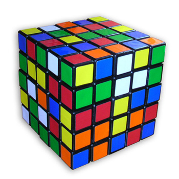
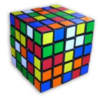
This is a 5x5 Rubik's cube, which has 25 little square faces making up a large face. As you increase the number of little cubes making up a Rubik's cube, the cube gets harder and harder to solve. Image: Mike Gonzalez, CC BY-SA 3.0.

Computer scientists determine whether a problem is easy or hard by calculating how long it would take to find its solution. There are many practical problems that fall within the "hard" category. This has important implications for which problems can be solved efficiently and precisely, and which ones can only be solved approximately. In other words, there is a limit to what can be computed in an exact and efficient way, and many practical problems require alternative, approximate solution methods. In theoretical terms the definition of hardness has led to one of the most intriguing open questions in mathematics, known as the P versus NP problem. So let's have a closer look at the concepts involved.

Easy problems

Every time you turn on the navigation system in your car, it invokes an algorithm to compute the shortest route between your current location and your desired destination. An algorithm is a well-defined and unambiguous sequence of instructions that can be performed by a computer (or, more precisely, a Turing machine), and which will return a result within a finite number of steps. Each step consists of a basic operation, such as comparing or adding two numbers, or looking up a stored value in the computer's memory. But when executed in a proper way, this sequence of simple operations eventually results in an answer, in this case the shortest route between two locations.

Not all algorithms are created equal, though. Some algorithms may be more efficient than others, that is, they return an answer more quickly. The efficiency of an algorithm is expressed in terms of the largest number of steps it might need on any (arbitrary) input to return an answer. This is called its worst-case running time.

Suppose, for example, you are given a sequence of $n$ distinct numbers in some random order, and you need to sort them from smallest to largest. It is quite easy to construct a simple sorting algorithm that will never need more than $\frac{1}{2}n (n-1)= \frac{1}{2}n^2-\frac{1}{2}n$ steps to do this. In the worst case you will need to compare each of the $n$ numbers with each of the $n-1$ other numbers, giving $n(n-1)$ comparisons. But since you don’t need to compare a given pair of numbers twice (when you have compared $a$ with $b$ you don’t need to compare $b$ with $a$ ) the $n(n-1)$ can be divided by $2$ . So, the worst-case running time of this simple sorting algorithm is $\frac{1}{2}n^2-\frac{1}{2}n$ steps. Generally, an algorithm that needs a maximum number of steps that grows proportional to $n^2$ is said to have a worst-case running time of $O(n^2)$ . The precise definition of this notation is given in the box.

Big O notation

Write $S(n)$ for the worst-case running time of a particular algorithm (e.g. putting a list of $n$ numbers into numerical order). If there are positive integers $m$ and $K$ so that for sufficiently large $n$ we have

$S(n) \leq Kn^ m,$

then the worst-case running time is said to be $O(n^ m)$ . This means that any worst-case running time that is a polynomial of degree $m$ in $n$ is said to be $O(n^ m)$ .

A worst-case running time that is of the form $O(n^ m)$ for some (finite) value of $m$ , is called a polynomial running time. For example, our simple sorting algorithm has a polynomial worst-case running time with $m=2$ . Even for very long sequences of numbers (i.e., large values of $n$ ), we can still expect to get a correctly sorted list within a reasonable number of steps (never more than $n^2$ , in this case). In fact, there exist even faster sorting algorithms with a worst-case running time of $O(nlog(n))$ .

The shortest path algorithm that is used in your car’s navigation system also has a polynomial worst-case running time (this can be proven mathematically). Given a road network with $n$ junctions, the shortest path between any two junctions can be computed in $O(n^2)$ steps. So, regardless of whether you need to drive from your home to the nearest grocery store or from New York to Los Angeles, you will not have to wait too long for your navigation system to compute the shortest route.

Problems for which an efficient algorithm (i.e., with a polynomial worst-case running time) can be constructed are considered "easy" problems. These easy problems together make up what is known in theoretical computer science as problem class P (for Polynomial). Thus, the sorting problem and the shortest path problem are both in this problem class P.

Yes or no?

As a technical aside, computational problems are usually stated as decision problems. In other words, rather than asking what the shortest route is between places $A$ and $B$ , we ask: is there a route between $A$ and $B$ that is of length at most $k$ ? This question has a yes/no answer, which is why it's called a decision problem. If your algorithm returns "yes" as an answer, it should also give at least one such route as an example, for which you can then easily check that its length is indeed not longer than $k$ .

This decision version of the shortest path problem can be directly converted into the version we had to start with, called the optimisation version. First, find an upper bound $K$ for the distance between $A$ and $B$ . One naive and easy-to-calculate upper bound is to simply add up the distances between all neighbouring pairs of the $n$ junctions in the road network (this is at most $n^2$ additions). Then ask the question: is there a route between $A$ and $B$ that is of length at most $K$ ? By construction of the upper bound $K$ , the answer will of course be "yes". So next ask the question: is there a route between $A$ and $B$ that is of length at most $K-1$ ? Continue this until for some value $l$ the answer is still "yes", but for $l-1$ it is "no". The shortest route between $A$ and $B$ will then obviously be of length $l$ (and your algorithm will have given you at least one such route).

If your algorithm for solving the decision version of the shortest path problem is efficient (i.e. has a worst-case running time that is polynomial in $n$ ), then the converted algorithm for solving the corresponding optimisation problem is also efficient. To see this for the given example, note that the upper bound $K$ is at most $d\times n^2$ , where $d$ is the largest distance between any neighbouring pairs of the $n$ points. So, we would need to run the decision version algorithm at most $dn^2$ times. Since the decision version algorithm has a worst-case running time of $O(n^2)$ , the optimisation version algorithm will have a worst-case running time of $O(n^4)$ , which is clearly still polynomial. However, as mentioned above, for the shortest path problem it is actually possible to construct an $O(n^2)$ algorithm to solve the optimisation version of the problem as well.

Hard problems

Unfortunately, not all computational problems are easy. Consider this simple extension of the shortest path problem. Given $n$ different cities and the distances between them, your job is to visit each of them exactly once and then return to your starting city, but in such a way that your total travel distance is as short as possible. So, the question is: in which order do you need to visit these $n$ cities so that the total length of your tour is as small as possible?

What's the shortest tour visiting all your favourite sites?

This problem is known as the travelling salesman problem (TSP). At first glance it seems very similar to the shortest path problem. However, so far nobody has been able to construct a polynomial-time algorithm for solving TSP optimally. In practice, the only way to guarantee to always find the shortest tour, for any given TSP instance, is to exhaustively evaluate all possible orderings of the $n$ cities, and then simply pick that ordering which results in the shortest tour.

However, the number of possible orderings of cities grows extremely fast with an increasing number of cities. In fact, the number of possible orderings is

$n! = n \times (n-1) \times (n-2) \times .. \times 2 \times 1.$

In practice, this means that every time you increase the number of cities $n$ by one, the number of possible city orderings more than doubles. So, the exhaustive evaluation algorithm has a worst-case running time that is at least $O(2^ n)$ — that's 2 multiplied by itself $n$ times — which is called exponential. (See this article for more details about comparing the running times, or computational complexity, of different algorithms.)

For example, for a problem instance with only five ( $n=5$ ) cities, there are 120 possible orderings, or tours. This is OK. But for $n=10$ cities, the number of possible tours is already over three million. And for $50$ cities it would take longer than the lifetime of the Universe to evaluate all possible tours, even for the fastest computers. Clearly, such an exhaustive algorithm is not efficient.

To appreciate the difference between a polynomial — e.g., $O(n^2)$ — and an exponential — e.g., $O(2^ n)$ – worst-case running time, take a look at the figure below. With increasing values of $n$ (along the horizontal axis), the polynomial running time (blue line) grows relatively slowly, but the exponential running time (red line) quickly goes through the roof. Problems such as TSP, for which only exponential-time algorithms (or worse) are available to solve them optimally, are appropriately called intractable — we may have to wait "forever" to get an answer.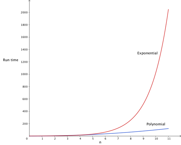

The blue line is the graph of the function n², a polynomial, and the red line is the graph of the exponential function 2ⁿ.

Hard, but easy to check

Amongst those intractable problems there is a special class of problems: those for which a solution, if it is somehow given, can still be checked efficiently. For example, consider the decision version of a TSP problem: is there a tour which visits all cities and has length at most $k$ ? Suppose someone told you the answer is "yes", and provided such a tour. It is then easy to check that its length is indeed not more than $k$ by simply adding up the individual distances between the cities along the given tour. If there are $n$ cities this requires $n$ additions, so a "yes" answer can be verified in polynomial time (regardless of how long it took to get that answer). Problems which have this property, together with the problems already in the P class, make up the larger problem class NP (for nondeterministic polynomial).

Very hard problems

A problem that is at least as hard as any problem in the NP class is called an NP-hard problem. NP-hard problems don't need to have solutions that can be checked efficiently, so they don't need to be in NP themselves. But those NP-hard problems that are themselves in NP form a special subclass: they are called NP-complete problems. If you are confused about all those problem classes, this diagram should help:

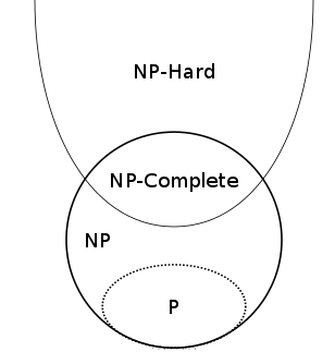
NP contains P and intersects the class of NP-hard problems. The intersection comprises the NP-complete problems. Image: Behnam Esfahbod, CC BY-SA 3.0.

To determine whether a given NP problem B is NP-complete, you need to show (mathematically) that it is at least as hard as some other problem A already known to be NP-complete. Simply put, if you can transform any instance of problem A to an equivalent instance of problem B, and that a solution to B then translates back into a solution to A, provided this transformation itself can be done in polynomial time, then problem B is also NP-complete. In mathematical terms, A reduces to B: A < B.

In 1971 the American computer scientist and mathematician Stephen Cook published a complicated proof to show that any problem in NP can be reduced to something called the Boolean satisfiability problem (or SAT). A similar proof was developed around the same time, but independently, by Leonid Levin in the (then) USSR. With this, the existence of the first known NP-complete problem was established.

Subsequently, Richard Karp proved an additional 21 common problems from computer science to be NP-complete, by reducing SAT to each of them. Since then, thousands of other problems have been shown to be NP-complete as well. TSP is one of them.

There is one caveat here. Even though nobody has been able to construct a polynomial-time algorithm for solving an NP-complete problem, it is mathematically not known whether this is really impossible. In other words, it is still an open question in theoretical computer science whether NP is strictly larger than P (i.e., there are indeed problems in NP that are not in P), or whether NP is actually the same as P. If the former is true then NP-complete problems really are hard. If the latter is true we simply have not yet been clever enough to find a polynomial-time algorithm to solve NP-complete problems. Given the practical evidence so far, the former seems most likely though. But the race is on among computer scientists and mathematicians to resolve this question formally, one way or the other. There is even a $1 million prize to be won. If, against expectations, P does turn out to be equal to NP then the diagram above collapses as follows:

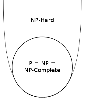
If NP turns out the equal to P then the diagram collapses. Image: Behnam Esfahbod, CC BY-SA 3.0.

Approximate solutions

NP-complete problems such as TSP are not just a theoretical issue. They show up all over the place: in telecommunications, logistics, engineering, scheduling, chip design, data security, and countless other day-to-day business applications. And these real-world problem instances often consist of hundreds or even thousands of "cities" (i.e., they have a large input size n). Highly intractable, unfortunately. So, there is a real limit to which practical problems can be solved in an exact and efficient way.

However, this does not mean that there is nothing we can do. In fact, for many real-world applications it is not always necessary to find the most optimal solution. For example, a travelling salesperson might not necessarily need the very shortest possible tour. A sub-optimal tour could still be adequate, as long as it does not exceed a given travel time or budget constraint. In other words, an approximate solution will still do fine in many practical situations, especially if such a sub-optimal solution can be found efficiently, i.e., in polynomial time.

So, it is worth trying to construct efficient approximation algorithms that find sub-optimal, but still "good enough", solutions to NP-complete problems. In computer science, such approximation algorithms are called heuristics. However, designing good heuristics can be more of an art than a science, and often comes down to just trial-and-error. You can find out more about this topic in this article on the Evolution Institute website, and we will also explore it in a future article on Plus.

About the author

Wim Hordijk is a computer scientist currently on a fellowship at the Institute for Advanced Study of the University of Amsterdam, The Netherlands. He has worked on many research and computing projects all over the world, mostly focusing on questions related to evolution and the origin of life. More information about his research can be found on his website.

Plus.Maths.org