Add new comment

What's the price for relaxing the rules?

After weeks of tight COVID-19 restrictions we could all do with a breather. Many businesses are being hit hard by a lack of pre-Christmas trade and the rest of us are longing for some time with friends and family. Surely we could afford a stretch of time in a lower tier, and then tighten up restrictions again later? What difference can a few days make?

The sad, but mathematically unshakeable, truth is "a lot". The graph below illustrates why. It shows, for realistic assumptions, how milder rules can allow a steep exponential growth of cases over a relatively short period of time (the rising part of the red curve), which can't be undone in the same amount of time using stricter rules (the declining part of the red curve). A few days of relative freedom come at the price of a longer time spent under tough interventions. This will lead to all the health costs for those who catch COVID-19 as a result. And even just focussing on the economic case, a delay to intervention is only beneficial in the very short term: a longer time will be probably be needed in a higher tier, or worse, another lockdown in future.

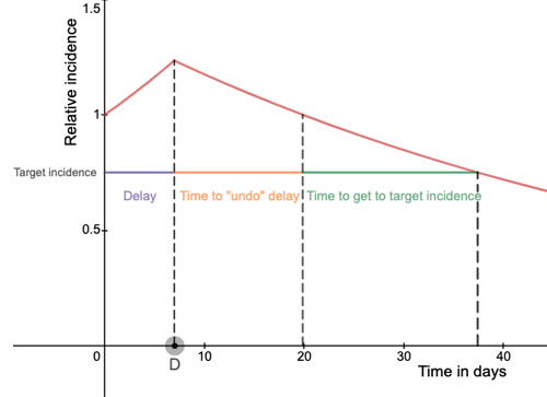
The red curve shows that rise in relative incidence under milder restrictions, and then the slow decline after tougher measures are brought in after seven days (on day D). The coloured intervals denote the various time periods involved in bringing the relative incidence down to a target value. The exact meaning of this graph is explained below.

To properly understand this graph, imagine that now, on day 0, we have two strategies. We can impose a set of tough rules straight away, or we can start with a set of milder rules and impose the tougher ones later on when things threaten to get out of hand again. Suppose that the milder rules result in a reproduction number $R=1.2$ and the tougher restrictions come with a value of $R=0.9$ . A value of $R$ greater than 1 for the mild set of rules means that they are not quite enough to control infection, while $R$ less than 1 for the tougher rules means that these are assumed to be strict enough to force the epidemic into decline.

See here for all our coverage of the COVID-19 pandemic.

We can predict how many people will become infected every day over the next few weeks using an exponential model — such models are suitable for the kind of time period we are looking at, and more than enough to illustrate the principles involved (if you are interested in the actual maths, see the end of the article). In practice reporting of cases would never look exactly like this as there would be a delay for detection, but here we plot the true state of the epidemic under this model.

The result is shown in the graph below, where the horizontal axis measures time in days, and the vertical axis measures the incidence of COVID-19: that's the number of new cases per day. However, it measures the incidence relative to the incidence we have today, at time 0. This means that the number shown for day $t$ is the total number of new cases on day $t$ , divided by the number of new cases on day 0. Suppose we impose the tougher rules on day $D.$ In the graph below we have set $D=7$ , so that's a delay of a week before imposing the tough rules, but you can use your mouse to move $D$ on the horizontal axis, to see what happens.

The red curve shows how the relative incidence changes over time. For comparison we have also included a blue dashed curve, which shows the change in relative incidence we'd get if we had introduced the tough rules straight away, on day $D=0$ .

Crucially, the red curve is not symmetric: the levelling off after day $D$ is slower than the sharp initial rise. It takes longer to get back to the relative incidence of 1 we started with than it takes to get from time 0 to day $D$ at which we see the peak of the red curve. This is typical for successful control measures for COVID-19 so far: they tend to be only just enough to keep the virus under control. What's more, the red curve never drops as low as the blue curve, which represents the scenario where tough rules are introduced straight away. So the delay we introduced can never be made up for.

We can make this even more concrete. Say our aim, today on day 0, is to reduce the incidence of COVID-19 to 75% of what it is now. How long would this take if we start with milder rules and introduce the tough ones on day $D$ ? The graph below shows that the time it takes to reach a relative incidence of 0.75 is divided into three time intervals. The first interval (purple in the graph below) is simply the delay $D$ . The second interval (orange) is the time it takes to "undo" the rise in cases allowed by the mild rules and get back to the initial relative incidence of 1. And the third interval (green) is the time it takes to get the relative incidence from 1 down to 0.75: it's the time we would have had to wait to get down to 0.75 if we had introduced the tough rules straight away.

If you do the maths (see the end of the article) you will see that, for the values of $R$ we are assuming, the second time interval (orange) is equal to $1.841 \times D.$ If there's a delay of a week, so $D=7$ , then $1.841 \times D \approx 13.$ So every seven days of relative freedom, will be paid for with 13 days — nearly two weeks — of stricter rules that are needed to get back down to the relative incident we started with.

Another thing the maths tells us is how the total number of COVID-19 cases we expect to see over a period of, say, six weeks depends on the delay of $D$ days before we impose the stricter rules. The result is shown in the graph below. The horizontal axis represents the delay $D$ and the vertical axis measures the total number of cases over six weeks (42 days) relative to the total number of cases we have at time 0. As you can see, the relative total number of cases at first increases with the delay $D,$ illustrating the price we pay for the delay in terms of people getting sick. Later on, for $D$ just over 30, the curve flattens off a little. This shows that once the delay is long enough, you can't make things much worse by making it even longer as the change to stricter measures is so near the end of the period we are counting cases over.

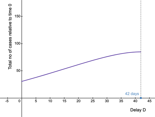
The total number of cases over six weeks (relative to the total number of cases at time 0) for the delay D varying from 0 to 42.

The lesson from all this is simple: a few days of relative freedom come at a heavy price in terms of the longer time we will need to spend under stricter rules later on, and in terms of the number of people who get sick. We just have to hang on a little while longer.

I want to see the maths!

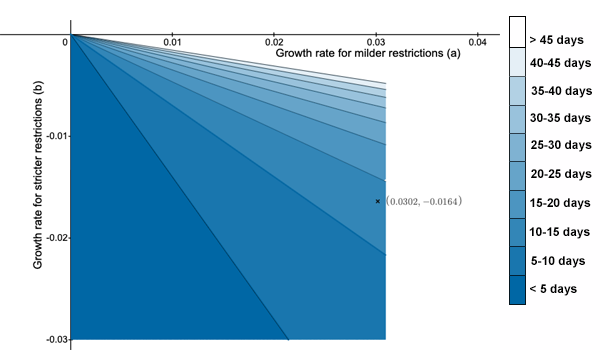
OK. Recall we assumed that the milder set of rules results in a reproduction number $R=1.2$ and that the tougher set of rules results in a reproduction number $R=0.9.$ The exponential model actually works with the growth rate, rather than the reproduction number, but as we have seen in a previous article, there's a way of working out the former from the latter. In our case, this gives a growth rate of $a = 0.0302$ for the mild rules and a growth rate of $b=-0.0164$ for the tough rules. The fact that the latter growth rate is negative reflects the fact that the rules are tough enough to force the epidemic into decline.

Our exponential model says that, before the tougher restrictions are imposed on day $D$ , the relative incidence $r(t)$ at time $t$ is

$r(t)=e^{a t}.$

So this expression applies for $0\leq t \leq D.$

Then for a time $t>D$ , so that’s after the tougher rules have been imposed, the relative incidence is

$r(t)=e^{a D + b(t-D)}.$

If you want to figure out how long it takes to reach a relative incidence of 0.75 with a delay of $D$ days before imposing the tougher rules, you need to solve

$r(t)=e^{a D + b(t-D)}=0.75$

for $t.$

You can do the maths for yourself, or simply believe that the answer is

$t= D -\frac{a}{b}D+\frac{\ln {(0.75)}}{a}.$

The terms in this sum represent the three time intervals mentioned above. In particular, the middle term represents the time needed to undo the exponential growth permitted by the mild rules that were in force for $D$ days, and get back to a relative incidence of 1. Note that, crucially, this term is independent of the relative incidence you are aiming at: whether you only want to get down to 90% of the incidence on day 0, or all the way down to 1%, a delay of $D$ days will always come at a price of $-a/b D$ days just to get back to a relative incidence of 1. The important piece of information here is the scaling factor of $-a/b.$

The 2D plot below shows the effect for a delay of $D=7$ for the various combinations of values of $a$ (on the horizontal axis) and $b$ (on the vertical axis). The shaded regions represent the extra amount of time in days that needs to be spent under stricter rules for a specific combination of $a$ and $b$ , from dark blue (five days or less) through to very light blue (between 40 and 45 days) and ultimately white (more than 45 days).

Substituting the growth rates we used above associated to the mild and the strict set of rules, $a = 0.0302$ and $b=-0.0164$ , gives

$-\frac{a}{b}D=1.841 \times D.$

For a delay of $D=7$ days this gives

$-\frac{a}{b}\times =1.841 \times 7 \approx 13.$

This corresponds to the point marked in the third shaded region (counting from the bottom) in the plot above.

So in this case a week of milder rules (i.e. being in a lower tier) comes at the price of nearly two weeks that will then need to be spent under stricter rules (e.g. in a higher tier), just to get back to where we started. That’s two weeks of less freedom for individuals and lost earnings for business.

Of course the delay also comes at a health cost. Let’s look at the total number $C(D)$ of cases over a period of $T_{max}$ days, relative to the total number of cases at time 0, and see how this depends on the delay $D$ (in our example above we considered a period of six weeks, so in that case $T_{max}=42$ days). The number $C(D)$ is equal to the integral of the incidence with respect to time

$C(D)=\int _{0}^{T_{max}}r(t)dt.$

Since $r(t)$ is a piecewise function this is the sum of two integrals,

$C(D)= \int _0^ D e^{b t} dt + \int _ D^{T_{max}} e^{b D + a(t-D)} dt.$

Integrating both integrals gives,

$T(D)=\left.\frac{e^{b t}}{b} \right]^ D_0 + e^{b D}\left. \left( \frac{e^{a(t-D)}}{a}\right) \right]^{T_{max}}_ D$

Evaluating the right hand side of this expression we get,

$T(D)= \frac{e^{a D}-1}{a} +e^{a D}\left(\frac{e^{b( T_{max}-D)} -1}{b}\right).$

Plotting this function for $T_{max}=42$ gives the following curve (also shown in the figure above):

The total number of cases over six weeks (relative to the total number of cases at time 0) for the delay D varying from 0 to 42.

About this article

Julia Gog. Photograph by Henry Kenyon.

Julia Gog, Professor of Mathematical Biology at the University of Cambridge, and Marianne Freiberger Editor of Plus, produced this article as part of a collaboration between Plus JUNIPER, the Joint UNIversity Pandemic and Epidemic Response modelling consortium. JUNIPER comprises academics from the universities of Cambridge, Warwick, Bristol, Exeter, Oxford, Manchester, and Lancaster, who are using a range of mathematical and statistical techniques to address pressing question about the control of COVID-19. You can see more content produced with JUNIPER here.

Gog is also a member of SPI-M, a modelling group which feeds its results into the Scientific Advisory Group for Emergencies (SAGE).

Plus.Maths.org

What's the price for relaxing the rules?

I want to see the maths!

About this article

Filtered HTML