It's one of the most beautiful sights in nature: fireflies illuminating the night with their synchronised flashing (see the video on the right). Something slightly less romantic, but equally magical, happens when you place two or more metronomes on a tray. No matter how different their beats were to start with, after a while they synchronise (you can watch 32 metronomes synchronise in the second video). In scientific jargon this phenomenon is known as phase locking. And thanks to mathematicians from the University of Liverpool and Imperial College, London, we've recently come a little closer to understanding the maths behind it.

Phase locking was first observed in the 17th century by Christiaan Huygens and has since been seen in a wide range of systems, including not only fireflies and metronomes, but also the interaction between rates of breathing and heartbeats in humans. In the 1960s the famous Russian mathematician Vladimir Arnol’d introduced a simple model to study phase-locking phenomena. The model is meant to describe a point moving periodically around a circle (representing one phase) with the motion being affected by an external force (representing the other phase). You can see the function that implements the model in the box below.

The model depends on two parameters, a and b: each pair of values of these parameters gives an individual function, and hence an individual model. So Arnol'd really introduced a whole family of models, one for each pair of values for a and b, known as the Arnol'd family. The family has been used as a simplified model for a large number of physical and biological systems, such as a beating heart.

The Arnol'd family

You can think of a circle as the interval from 0 to 1 with the end-points glued together. So each point on the circle can be represented by a number t between 0 and 1. The Arnol'd family is given by functions of the form

This gives a dynamical system: a point moves to then moves to , which in turn moves to and so on.

Each model in the Arnol'd family represents a dynamical system (a point moving around a circle). One question mathematicians like to ask about dynamical systems is what happens when you change one or both of the parameters that describe it ever so slightly: does the overall behaviour of the system remain roughly the same, or does it change dramatically? This is an important question for real world systems. For example, if it's the interaction of heart beat and breathing you are looking at, you'd want to know whether the system remains stable under a small change in the parameter that describes either of the two, or whether such a change would cause it to go "wild".

For the Arnol'd family we can capture this idea in a picture. Each point in the image below corresponds to a different choice of parameters, with the rotation parameter drawn horizontally and the parameter representing the external force vertically. White regions indicate parameter pairs where phase-locking phenomena lead to a system that is stable (ie, it doesn't change drastically) when the parameters are changed slightly. Experiments had suggested that this stable behaviour can be found everywhere on the picture: even if no white area is visible in some region at first, if you zoom in on it, one will eventually be revealed. (In mathematical language, stable behaviour is dense.)

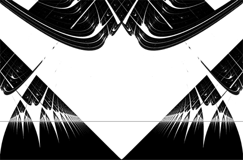
Each point on this picture has coordinates (a,b), where a and b are the parameters in the Arnol'd family. Points in the white region are those for which the corresponding model is stable under small changes.

When the forcing parameter is small (more precisely: for parameters below the grey line in the picture), this density of stable behaviour was already verified and explained by Arnol'd. The general case remained open for more than 40 years – but has now been solved by Lasse Rempe-Gillen (University of Liverpool) and Sebastian van Strien (Imperial College).

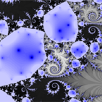
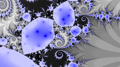
Their proof relies on an extension of the model that produces another very pretty picture. Each model is represented by a point moving around a circle, which itself sits in the two-dimensional plane. It is possible to extend each model to the whole plane, so rather than points moving on a circle you're looking at points moving around in the plane (this extension uses complex numbers). The image below shows the behaviour of points in the plane for a particular Arnol'd model (a particular choice for the parameters a and b). The grey areas are the Julia set of the corresponding function, points here are moved around by the model in a chaotic fashion (you can find more about Julia sets here). Points that are not part of the Julia set are moved around in a more regular manner.

Each point on this picture has coordinates (a,b), where a and b are the parameters in the Arnol'd family. Points in the white region are those for which the corresponding model is stable under small changes.

The result has been accepted for publication in the Duke Mathematical Journal.