
Maths in a minute: The logistic map
The logistic map is famous for two reasons: it gives a way of predicting how a population of animals will grow or shrink over time, and it illustrates the fascinating phenomenon of mathematical chaos.

How many of these will you have after a month? Photo: lens-flare.de, CC BY-NC 2.0.
Imagine you have an aquarium big enough to hold 100 guppies, those tiny and colourful little fish that love breeding. The question is, how many guppies can you expect to have next month if you let them get on with it?
The answer will, in part, depend on how many guppies you have to start with. If you are far away from maximal capacity of 100 guppies, so there's plenty of food and space for everyone, the population next month is likely to be bigger. If you're very near the maximal capacity, so that there's not enough food and space to go around, then the population is likely to decrease.
The logistic map takes account of the idea that the growth of the population depends on how many animals there are to start with. Write $x$ for the proportion of the maximal capacity of the tank that are alive today. So if $x=1/2$ then in our example there are 50 guppies, if $x=1/4$, then there are 25 guppies, if $x=0$ there are no guppies, and of $x=1$ then the maximal capacity of 100 guppies are alive. Then the logistic maps suggests that next month the population size (as a proportion of the maximal guppy capacity of the tank) will be $$rx(1-x).$$Here $r$ is a number you might think of as the growth rate of the population, which depends on things like how many guppies are generally born in a month and how many die. We won't go into how you would calculate $r$, or why the formula above is a good estimate of next month's size of the population, because here we want to focus on the mathematical properties of the logistic map. You can find out more about these questions here.
As an example, if the growth rate is $r=4$ and the proportion of maximal capacity this month is $x=0.7$, then the logistic map says that next month the proportion will be $$4 \times 0.7(1-0.7)=4 \times 0.7 \times 0.3 = 0.84.$$ So if the maximal capacity is 100 guppies, then next month you will have 84 guppies.Notice that given the formula above, you can estimate, not just the size of the population next month, but also the size further in the future. Applying the formula to the current proportion $x$ of guppies alive today gives you the proportion for next month. Applying the formula again to that new proportion, gives you a proportion for two months from now. Then applying it again gives a proportion for three months from now, and so on.
As an example, assume the growth rate is $r=4$ and that we start with a proportion of $x=0.7$ of the maximal capacity. The graph below shows how the population size changes over the first five months, according to the logistic formula. Notice that when the population has nearly reached maximal capacity in month 3 it plummets to nearly zero the month after — the overcrowding has taken its toll.
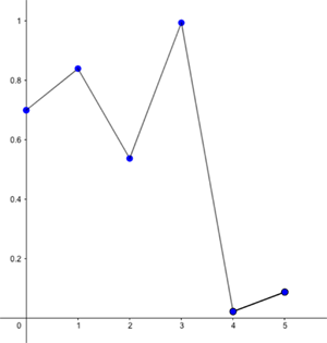
Predictions for proportion of maximal capacity alive (vertical axis) for the first 5 months (horizontal axis), for r=4 and initial proportion x=0.7.
In theory we could go on like that forever, using the logistic expression to estimate the size of the population very far into the future. That involves a lot of calculations though, so the question is if we can say something more general, without going into the details.
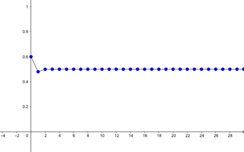
The answer is "sometimes you can" — it all depends on the value the growth rate $r$ takes. It turns out that if $r$ is smaller than 1, then the growth rate is just too small to keep the population going, and it will eventually die out. This is true no matter how big the population was to start with. Even if you start with the maximum of 100 guppies ($x=1$), eventually there won't be any left. You can see this in the examples below, where we have $r=0.9. $ The first graph shows the evolution of the population if the initial proportion is $x=0.7$ and the second if we have $x=0.4$.
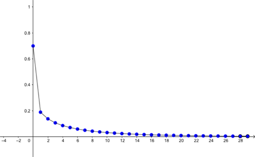
Predictions for proportion of maximal capacity alive (vertical axis) for the first 30 months (horizontal axis), for r=2 and initial proportion x=0.7. Eventually the population dies out.
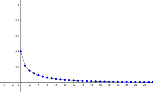
Predictions for proportion of maximal capacity alive (vertical axis) for the first 30 months (horizontal axis), for r=2 and initial proportion x=0.4. Eventually the population dies out.
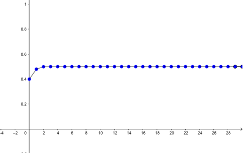
Predictions for proportion of maximal capacity alive (vertical axis) for the first 30 months (horizontal axis), for r=2 and initial proportion x=0.4. Eventually the proportion alive settles down to (r-1)/r=1/2.
Predictions for proportion of maximal capacity alive (vertical axis) for the first 30 months (horizontal axis), for r=2 and initial proportion x=0.6. Eventually the proportion alive settles down to (r-1)/r=1/2.
As you increase $r$ through 3, you will find that the proportion of the maximal capacity no longer settles down around one specific value. But its behaviour is still quite predictable: instead of homing on a specific size, the population will periodically move up and down around several different values. This happens for almost all starting values $x$ (you can find out more about this periodic behaviour here).
You can see this in the examples below, where we have taken $r=3.5.$ The first graph shows the evolution of the population if the initial proportion is $x=0.6$ and the second if we have $x=0.3$.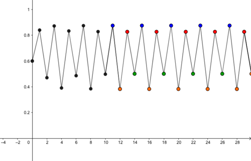
Predictions for proportion of maximal capacity alive (vertical axis) for the first 30 months (horizontal axis), for r=3.5 and initial proportion x=0.6. Eventually the population size settles into to a periodic pattern, moving between four different values (shown in different colours).
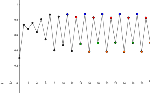
Predictions for proportion of maximal capacity alive (vertical axis) for the first 30 months (horizontal axis), for r=3.5 and initial proportion x=0.3. Eventually the population size settles into to a periodic pattern, moving between four different values (shown in different colours).
So far the behaviour of the population, as estimated by the logistic map, was nicely predictable: it settled down into a predictable pattern, and this pattern didn't depend on what value of $x$ you started with. However, all hell breaks loose once the growth rate moves through a particular value, close to 3.56995.
For most values of $r$ at or beyond the ominous 3.56995 the population may never settle down into a predictable pattern. But that's not the worst: two different starting values of $x$ can lead to wildly different predictions of the future, even if they are very, very close. You can see this below for the example of $r=4.$ The first graph takes the initial proportion to be $x=0.6$ and the second takes $x=0.62$. Although these two values are close, the population size behaves differently in the future.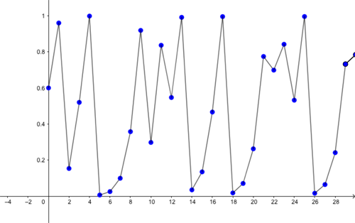
Predictions for proportion of maximal capacity alive (vertical axis) for the first 30 months (horizontal axis), for r=4 and initial proportion x=0.6.

Predictions for proportion of maximal capacity alive (vertical axis) for the first 30 months (horizontal axis), for r=4 and initial proportion x=0.62. although this is very close to the starting proportion of 0.62 above, the population evolves differently.
This latter fact, that different starting values can lead to wildly different futures, makes prediction really difficult. If you miscalculate your starting population, for example because one guppy is hiding behind the water tank so you don't count it, then your prediction could be as good as useless.
This phenomenon, where arbitrarily close to any starting value there are other values that lead to vastly different predictions over time, is known as sensitive dependence on initial conditions or the butterfly effect. The effect is the hallmark of mathematical chaos (for a precise mathematical definition, see here).
It's not only the logistic map that exhibits sensitive dependence on initial conditions, but also many other mathematical expressions, such as those used to predict the weather. This is why many real-life systems are so hard to predict. What makes the logistic map special is that it's a relatively simple mathematical expression. So chaos can ensue even when the underlying system is not particularly complex.
Finally we should note that, for the logistic map, not all values of $r$ beyond 3.56995 lead to an expression that exhibit chaos. There are some isolated ranges of values for $r$ for which things become predictable again. These ranges go by the soothing name of islands of stability.
You can find out more about chaos in these Plus articles.