Can science be used to further our understanding of art? This question triggers reservations from both scientists and artists. However, for the abstract paintings produced by Jackson Pollock in the late 1940s, the answer is a resounding "yes".

Pollock dripped paint from a can on to vast canvases rolled out across the floor of his barn. Although recognised as a crucial advancement in the evolution of modern art, the precise quality and significance of the patterns created by this unorthodox technique remain controversial. Here we analyse Pollock's patterns and show that they are fractal - the fingerprint of Nature.

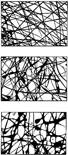
Figure 1: Detail of non-chaotic (top) and chaotic (middle) drip trajectories generated by a pendulum and detail of Pollock's 'Number 14' painting from 1948 (bottom).

In contrast to the broken lines painted by conventional brush contact with the canvas surface, Jackson Pollock used a constant stream of paint to produce a uniquely continuous trajectory as it splattered on to the canvas below. A typical canvas would be reworked many times over a period of several months, with Pollock building a dense web of paint trajectories. This repetitive, cumulative, "continuous dynamic" painting process is strikingly similar to the way patterns in Nature evolve.

Other parallels with natural processes are also apparent. Gravity plays a central role for both Pollock and Nature. Furthermore, by abandoning the easel, the horizontal canvas became for Pollock a physical terrain to be traversed. His approach in working from all four sides replicated the isotropy (having the same properties in all directions) and homogeneity of many natural patterns. His canvases were also large and unframed, similar to a natural environment. Can these shared characteristics be the signature of a deeper common approach?

Since its discovery in the 1960s, chaos theory has experienced spectacular success in explaining many of Nature's processes. Could Pollock's painting process therefore also be chaotic?

There are two revolutionary aspects to Pollock's application of paint and both have potential to introduce chaos. The first is his motion around the canvas. In contrast to traditional brush-canvas contact techniques, where the artist's motions are limited to hand and arm movements, Pollock used his whole body to introduce a wide range of length scales into his painting motion. In doing so, Pollock's dashes around the canvas possibly followed Levy flights: a special distribution of movements, first investigated by Paul Levy in 1936, which has recently been used to describe the statistics of chaotic systems.

The second revolutionary aspect concerns his application of paint by letting it drip on to the canvas. In 1984, a study of a dripping tap showed that small adjustments could change the falling fluid from a non-chaotic to chaotic flow, and Pollock could have likewise mastered a chaotic flow.

To investigate this possibility, a simple system can be designed to generate drip trajectories where the degree of chaos can be tuned. The system consists of a pendulum which records its motion by dripping an identical paint trajectory on to a horizontal canvas positioned below. When left to swing on its own, the pendulum follows a predictable, non-chaotic motion. However, by knocking the pendulum at a frequency slightly lower than the one at which it naturally swings, the system becomes a "kicked rotator".

By tuning the kick (which can be applied very precisely using, for example, electromagnetic driving coils), chaotic motion can be generated. Example sections of non-chaotic (top) and chaotic (middle) drip paintings are shown in Fig. 1. Since Pollock's paintings are built from many criss-crossing trajectories, these pendulum paintings like-wise feature a number of trajectories generated by varying the launch conditions. For comparison, the bottom picture is a section of Pollock's dripped trajectories.

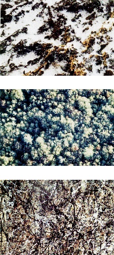
Figure 2: Photographs of (top) a 0.1m section of snow on the ground, (middle) a 50m section of forest and (bottom) a 2.5m section of Pollock's 'One: Number 31' painted in 1950.

A striking visual similarity exists between the drip patterns of Pollock and those generated by a chaotic drip system. If both drip patterns are generated by chaos, what common quality would be expected in the patterns left behind? Many natural chaotic systems form fractals in the patterns that record the process.

Nature builds its fractals using statistical self-similarity: the patterns observed at different magnifications, although not identical, are described by the same statistics. The results are visually more subtle than the instantly identifiable, artificial patterns generated using exact self-similarity, where the patterns repeat exactly at different magnifications.

Fortunately, there are visual clues which help to identify statistical self-similarity. The first relates to "fractal scaling". The visual consequence of obeying the same statistics at different magnifications is that it becomes difficult to judge the magnification and hence the length scale of the pattern being viewed. This is demonstrated in Fig. 2(top) and Fig.2(middle) for Nature's fractal scenery and in Fig. 2(bottom) for Pollock's painting.

A second visual clue relates to "fractal displacement", which refers to the pattern's property of being described by the same statistics at different spatial locations. As a visual consequence, the patterns gain a uniform character and this is confirmed for Pollock's work in the upper inset of Fig. 3, where the pattern density $P$ is plotted as a function of position across the canvas (logs are base 10).

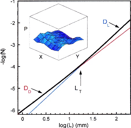
Figure 3: A plot of log N(L) versus log L for the aluminium trajectories of the painting 'Blue Poles'. The black line is the data (composed of 1523 data points within the first decade). The red and blue lines indicate the two gradients. Note that the graph remains linear beyond the range shown. The upper inset shows a plot of pattern density P versus the X and Y positions across the painting 'Number 14' (0.57m by 0.78m). P is defined as the per centage of the canvas surface area fill ed by the pattern within a square of side length L= 0.05m. The plotted ranges are 0 < P < 100% and 0< X, Y < 0.43m. The lower inset is a schematic representation of the box counting technique (see text for details).

These visual clues to fractal content can be confirmed by calculating the fractal dimension D of Pollock's drip paintings. The large amount of repeating structure within a fractal pattern causes it to occupy more space than a one dimensional line but not to the extent of completely filling the two dimensional plane. To detect and quantify this intermediate dimensionality of fractals, we calculate D using the well-established "box-counting" method.

In this method, we cover the scanned photograph of a Pollock painting with a computer-generated mesh of identical squares. The number of squares $N(L)$ which contain part of the painted pattern is then counted. This count is repeated as the size $L$ of the squares in the mesh is reduced. In this way the amount of canvas filled by the pattern can be compared at different magnifications. \par The largest size of square is chosen to match the canvas size ($L=2.08m$) and the smallest is chosen to match the finest paint work ($L=0.8mm$). Within this size range, the count is not affected by any measurement resolution limits (for example those associated with the photographic or scanning procedures). $D$ values are then extracted from a graph, such as the one shown in Fig. 3, using the relationship $N(L) \~ L_{-D}$. In Fig. 3, $N_T$ varies from 100 to $4x10^6$ squares over the shown $L$ range. The straight lines reflect the statistical self-similarity of the pattern and $D$ is calculated from the gradients.

The two chaotic processes proposed for generating Pollock's paint trajectories - Pollock's body motions and the dripping fluid motions - operate across distinctly different length scales. These scales can be estimated from film and still photography of Pollock's painting process. \par Based on the physical range of his body motions and the canvas size, his Levy flights over the canvas are expected to cover the approximate length scales $1cm < L < 2.5m$. In contrast, the drip process is expected to shape the trajectories over the approximate scales $1mm < L < 5cm$. This range is calculated from variables which affect the drip process (such as paint velocity and drop height) and those which affect paint absorption into the canvas surface (such as paint fluidity and canvas porosity). \par We would therefore expect the fractal analysis to reveal two $D$ values at different ranges, and Fig. 3 shows this to be the case. We label these as the drip fractal dimension $D_D$ and the Levy flight fractal dimension $D_L$. We note that systems described by two or more $D$ values are not unusual: trees and bronchial systems are common examples in Nature. \par A consequence of multiple $D$ values is that each value can be observed over only a limited range of scales. Recently, it has been stressed that so-called "limited range" fractals are no less fractal than ones observed over many orders of magnitude. Furthermore, a survey of fractals measured in physical systems indicates that the average range over which fractals are observed is approximately one order of magnitude. The range over which $D_D$ is measured is 1.1 - 1.3 orders (depending on the painting being analysed) and $D_L$ is measured over 2 orders. The length scale $L_T$ which marks the transition between $D_D$ and $D_L$ occurs at typically 1 - 5cm. These ranges are consistent with the values calculated above from their respective chaotic processes. \par The analysis of Fig. 3 produces $D_D=1.63$. For comparison, we note that typical $D$ values for natural fractal patterns such as coastlines and lightning are 1.25 and 1.3. Our analysis also shows that Pollock refined his dripping technique, with $D_D$ increasing steadily through the years. "Composition with Pouring II", one of his first drip paintings of 1943, has a $D_D$ value close to 1. "Number 14" (1948), " Autumn Rhythm" (1950) and "Blue Poles" (1952) have values of 1.45, 1.67 and 1.72. In each case, the value of $D_L$ was closer to 2 than $D_D$, indicating a more efficient space-filling fractal pattern at the larger scales. \par How did Pollock construct and refine his fractal patterns? In many paintings (though not all), he introduced the different colours more or less sequentially: the majority of trajectories with the same colour were deposited during the same period in the painting's evolution. To investigate how Pollock built his fractal patterns, we have therefore electronically de-constructed the paintings into their constituent coloured layers and calculated each layer's fractal content. \par We find that each of the individual layers consist of a uniform, fractal pattern. As each of the coloured patterns is re-incorporated to build up the complete pattern, the fractal dimension of the overall painting rises. Thus the combined pattern of many colours has a higher fractal dimenion than those of the individual coloured contributions. \par The layer he painted first plays a pivotal role - it has a significantly higher $D$ value than subsequent layers. This layer essentially determines the fractal nature of the overall painting, acting as an anchor layer for the subsequent layers which then fine tune the fractal dimension. A comparison between the anchor layer and the corresponding complete painting is shown in Fig. 4.

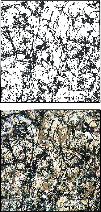
Fig. 4: A comparison of (left) the black anchor layer and (right) the complete pattern consisting of four layers (black, brown, white and grey on a beige canvas) for the painting 'Autumn Rhythm: Number 30' (2.66m by 5.30m) painted in 1950. The complete pattern occupies 47% of the canvas surface area. The anchor layer occupies 32%.

Pollock died in 1956, before chaos and fractals were discovered. It is highly unlikely, therefore, that Pollock consciously understood the fractals he was painting. Nevertheless, his introduction of fractals was deliberate. For example, the colour of the anchor layer was chosen to produce the sharpest contrast against the canvas background and this layer also occupies more canvas space than the other layers, suggesting that Pollock wanted this highly fractal anchor layer to visually dominate the painting. \par Furthermore, after the paintings were completed, he would dock the canvas to remove regions near the canvas edge where the pattern density was less uniform. He also took steps to perfect the "drip and splash" technique itself. His initial drip paintings of 1943 consisted of a single layer of trajectories which, although distributed across the whole canvas, only occupied 20\% of the $0.35m_2$ canvas area. By 1952 he was painting multiple layers of trajectories which covered over 90\% of his $9.96m_2$ canvas. This increase in both canvas size and density of trajectories was accompanied by a rise in the pattern's fractal dimension from 1 to 1.72. \par Finally we note that, because $D$ follows such a distinct evolution with time, the fractal analysis could be employed as a quantitative, objective technique to both validate and date Pollock's drip paintings. In conclusion, Pollock's contribution to the evolution of art is secure. He described Nature directly. Rather than mimicking Nature, he adopted its language - fractals - to build his own patterns.

Richard P. Taylor, Adam P. Micolich and David Jonas,

School of Physics, University of New South Wales, Sydney, 2052, Australia.

This article first appeared in Physics World, Volume 12, Issue 10, October 1999.

This content now forms part of our collaboration with the Isaac Newton Institute for Mathematical Sciences (INI) – you can find all the content from our collaboration here. The INI is an international research centre and our neighbour here on the University of Cambridge's maths campus. It attracts leading mathematical scientists from all over the world, and is open to all. Visit www.newton.ac.uk to find out more.