Unveiling the Mandelbrot set
Back in the 1970s and 1980s, mathematicians working in an area called dynamical systems made use of the ever-advancing computing power to draw computer images of the objects they were working on. What they saw blew their minds: fractal-like structures whose beauty and complexity is only rivalled by Nature itself. At the heart of them lay the Mandelbrot set, which today has achieved fame even outside the field of dynamics. This article describes where it comes from and explores its infinite intricacies.
Iteration
The Mandelbrot set is generated by what is called iteration, which means to repeat a process over and over again. In mathematics this process is most often the application of a mathematical function. For the Mandelbrot set, the functions involved are some of the simplest imaginable: they all are what is called quadratic polynomials and have the form f(x) = x2 + c, where c is a constant number. As we go along, we will specify exactly what value c takes.
To iterate x2 + c, we begin with a seed for the iteration. This is a number which we write as x0. Applying the function x2 + c to x0 yields the new number
Now, we iterate using the result of the previous computation as the input for the next. That is
and so forth. The list of numbers x0, x1, x2,... generated by this iteration has a name: it is called the orbit of x0 under iteration of x2 + c.
The theory of iterated functions is motivated by questions from real life. Modelling the growth of a population of animals is an example. The size of the population after one breeding cycle depends on how many animals there are at present, so mathematical models of population growth typically consist of a function f in a variable x, where x represents the present population size, and f(x) gives the expected population size after one breeding cycle. To work out the size of the population after any number of breeding cycles you need to iterate the function. Incidentally, the functions used in a standard model of population growth are quadratic polynomials very similar to the ones we will consider here, and this is what first motivated their study.
This leads to one of the principal questions in this area of mathematics: what is the fate of typical orbits? Do they converge or diverge? Do they cycle or behave erratically? The Mandelbrot set is a geometric version of the answer to this question.
Let's begin with a few examples. Suppose we start with the constant c = 1. Then, if we choose the seed 0, the orbit is
and we see that points in this orbit get bigger and bigger — the orbit tends to infinity.
As another example, choose c = 0. Now the orbit of the seed 0 is quite different: it remains fixed for all iterations.
If we now choose c = -1, something else happens. For the seed 0, the orbit is
Here we see that the orbit bounces back and forth between 0 and -1. This is a cycle of period 2.
To understand the fate of orbits, it is most often easiest to proceed geometrically: a time series plot of the orbit often gives more information about its fate. In the plots below, we have displayed the time series for x2 + c where c = -1.1, -1.3, -1.38, and 1.9. In each case we have computed the orbit of 0 and marked the points in it by dots which are connected by straight line segments. Note that the fate of the orbit changes with c. For c = -1.1, we see that the orbit approaches a 2-cycle. For c = -1.3, the orbit tends to a 4-cycle. For c = -1.38, we see an 8-cycle. And when c = -1.9, there is no apparent pattern for the orbit; mathematicians use the word chaos for this phenomenon.
Figure 1: the orbit of 0 for iteration of x2 - 1.1 . The orbit approaches a 2-cycle.
Figure 2: the orbit of 0 for iteration of x2 - 1.3. The orbit approaches a 4-cycle.
Figure 3: the orbit of 0 for iteration of x2 - 1.38. The orbit approaches an 8-cycle.
Figure 4: the orbit of 0 for iteration of x2 - 1.9. There is no apparent pattern, we see chaos.
To see additional time series plots for other values of c, select a c value from the options below:
- c = -0.65 (Tends to a fixed point)
- c = -1.6 (Chaotic behaviour)
- c = -1.75 (Tends to period 3)
- c = -1.8 (Chaotic behaviour close to 3-cycle, sometimes called intermittency)
- c = -1.85 (Chaotic behaviour)
- c = 0.2 (Tends to a fixed point).
Before proceeding, let us make a seemingly obvious and uninspiring observation. Under iteration of x2 + c, either the points in the orbit of 0 get larger and larger so that the orbit tends to infinity, or they do not. When the orbit does not go to infinity, it may behave in a variety of ways. It may be fixed or cyclic or behave chaotically, but the fundamental observation is that there is a dichotomy: sometimes the orbit goes to infinity, other times, it does not. The Mandelbrot set is a picture of precisely this dichotomy in the case where 0 is used as the seed. Thus the Mandelbrot set is a record of the fate of the orbit of 0 under iteration of x2 + c: the numbers c are represented graphically and coloured a certain colour depending on the fate of the orbit of 0.
Complex numbers
How, then, is the Mandelbrot set a picture in the plane, rather than on the number line on which all the c-values we have considered lie? The answer is, instead of considering only real values of c, we also allow c to be a complex number. If you are not familiar with complex numbers, then read this brief introduction or read Plus article Curious quaternions for more detail.
Let's look at some examples of the iteration of x2 + c when c is a complex number: if c=i, then the orbit of 0 under x2 + i is given by
and we see that this orbit eventually cycles with period 2. If we change c to 2i, then the orbit behaves very differently
and we see that this orbit tends to infinity in the complex plane (the numbers comprising the orbit recede further and further from the point 0, which has co-ordinates (0,0)). Again we make the fundamental observation that either the orbit of 0 under x2 + c tends to infinity, or it does not.
The Mandelbrot set
The Mandelbrot set puts some geometry into the fundamental observation above. Here is its precise definition:
The Mandelbrot set consists of all of those (complex) c-values for which the corresponding orbit of 0 under x2 + c does not escape to infinity.
Figure 5: the black region is the Mandelbrot set — pick any c-value from this black reason and you will find that when you iterate x2+c the orbit of zero does not escape to infinity. The Mandelbrot set is symmetric with respect to the x-axis in the plane, and its intersection with the x-axis occupies the interval from -2 to 1/4. The point 0 lies within the 'main cardioid', and the point -1 lies within the 'bulb' attached to the left of the main cardioid.
From our previous calculations, we see that c = 0, -1, -1.1, -1.3, -1.38, and i all lie in the Mandelbrot set, whereas c = 1 and c = 2i do not. We will represent the Mandelbrot set by the letter M. It is named after the mathematician Benoit Mandelbrot who was one of the first to study it in 1980.
At this point, a natural question is: why would anyone care about the fate of the orbit of 0 under x2 + c? Why not the orbit of i? Or 2 + 3i? Or any other seed, for that matter? As we will see below, there is a very good reason for inquiring about the fate of the orbit of 0; amazingly, the orbit of 0 somehow tells us a tremendous amount about the fate of all other orbits under x2 + c.
We remark at this point that our definition of the Mandelbrot set gives quite an easy way of drawing it using a computer, which is described in the Plus article Computing the Mandelbrot set.
Bulbs and antennas
Computer images of the Mandelbrot set, like the one above, give a hint of how incredibly intricate it is. It is known that, no matter how closely you zoom in on its boundary, it will always appear just as crinkly as it did before. The exact nature of the boundary's crinkliness is still one of the major open questions in maths. There are, however, quite a lot of things we can say about the Mandelbrot set, and these things reveal that its structure is by no means co-incidental: every little piece of it is loaded with mathematical meaning.
So let's have a close look at it. You can see that it consists of a main body, which looks a bit like a heart lying on its side and is therefore called the main cardioid of M (from the Greek kardia, meaning heart). Attached to the main cardioid are myriad "decorations". Closer inspection of these shows that all of them are different in shape.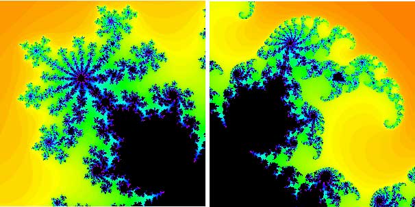
Figure 6: decorations of the Mandelbrot set in close-up. The two 'bulbs' shown here are directly attached to the main cardioid.
The decorations directly attached to the main cardioid in M are called primary bulbs or primary decorations. Any primary bulb in turn has infinitely many smaller decorations attached, as well as what appear to be antennas. In particular, as is clearly visible in figure 6, the "main antenna" attached to each decoration seems to consist of a number of spokes which varies from decoration to decoration.
There is a beautiful relationship between the number of spokes on these antennas and the dynamics of x2 + c for c lying inside the primary bulb. To see this, let's take a c value inside the big bulb that is attached to the main cardioid on the left, for example c=-1.01. Starting with the seed 0.0099, you can calculate that this function has a cycle of period two:
The point c = -1.01 is marked in white..
The Mandelbrot set keeps track of the orbit of 0, and if we use 0 as a seed we get:
x1 = -1.01,
x2 = 0.0101,
x3 = -1.00989799,
x4 = 0.00989395,
x5 = -1.00990210,
x6 = 0.00990227,
This is the case not only for c=-1.01: for any c value that lies inside the same bulb as -1.01 the function x2 + c has a 2-cycle and the orbit of zero is attracted to it.
Something similar happens for every primary bulb: if c lies in the interior of such a primary bulb, then the orbit of 0 is attracted to a cycle of some period n. The number n is the same for any c inside this primary bulb, and it is called the period of the bulb. To see that this is really true, open the Mandelbrot set iterator applet on my website, which was written by James Denvir. Clicking on a point in the Mandelbrot set shown in this applet will display the orbit of zero on the left. You will see that after a few iterations this orbit cycles.
Using the applet you can verify that the periods of some of the larger primary bulbs are as shown in figure 7. Simply click on a c-value inside a bulb and count the number of points in the cycle.
Figure 7: the periods of the bulbs
Figure 8 shows close-ups of the period 3, 4, 5 and 7 bulbs (in clockwise order starting from the top left). Now count the spokes of the largest antenna attached to each bulb (don't forget to count the spoke emanating from the primary bulb to the main junction point of the antenna.) What we are beginning to see here is a remarkable relationship: the number of spokes is precisely the period of the primary bulb!
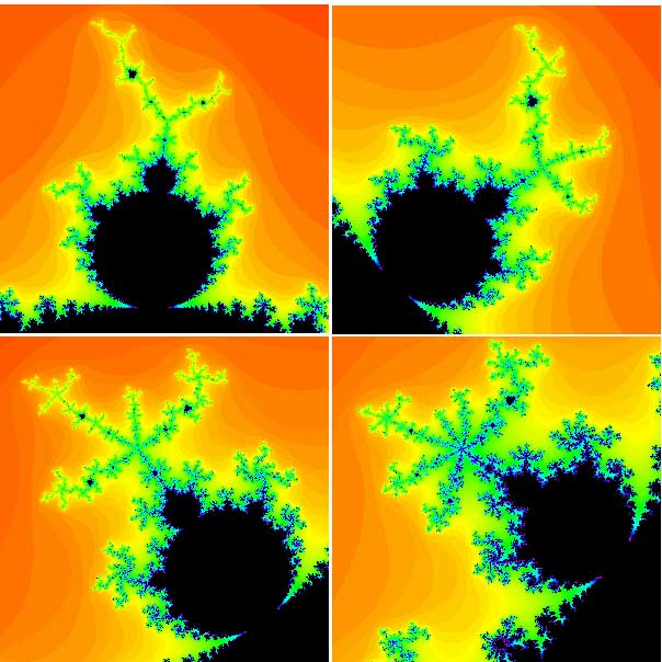
Figure 8: various bulbs and their periods. Clockwise from top left: period 3 bulb, period 4 bulb, period 7 bulb, period 5 bulb. Note that the period of the bulb is equal to the number of spokes on the main antenna.
A similar result is true for non-primary bulbs that are not directly attached to the main cardioid. In this case, the period of the bulb is a multiple of the number of spokes attached to its antenna.
Filled Julia sets
But the remarkable relationships don't end here. There is a second, more dynamic way to calculate the periods of these primary bulbs in M. To explain this, we have to introduce the notion of a filled Julia set. The filled Julia set for x2 + c is subtly different from the Mandelbrot set. For M, we calculated only the orbit of 0 for each c-value and then displayed the result. A c-value lies in M if the corresponding orbit of 0 does not escape to infinity. The Mandelbrot set is a picture in the c-plane.
For the filled Julia sets, we fix a c-value and then consider the fate of all possible seeds for that fixed value of c. Those seeds whose orbits do not escape form the filled Julia set of x2 + c. Putting it formally:
Fix a value of c. The filled Julia set of x2 + c is the collection of seeds whose orbit does not tend to infinity.
(Caution: There is also a notion of the Julia set. This term is used to describe the boundary of the filled Julia set.)From our examples above we see that the point 0 lies in the filled Julia set of x2 + 0, because it is fixed and does not go anywhere. But 0 is not in the filled Julia set of x2 + 1, because it escapes to infinity.
Thus, we get a different filled Julia set for each different choice of c. We write Jc for the filled Julia set of x2 + c. In figures 9 to 12 we have displayed the filled Julia sets for a variety of c-values.
Figure 9: the filled Julia set for c = -1.037 + 0.17i, which lies in a period 2 bulb.
Figure 10: the filled Julia set for c = -0.52 + 0.57i, which lies in a period 5 bulb.
Figure 11: the filled Julia set for c = 0.295 + 0.55i, which lies in a period 4 bulb.
Figure 12: the filled Julia set for c = -0.624 + 0.435i, which lies in a period 7 bulb.
To get a feel for filled Julia sets, see if you can show that the filled Julia set for c = 0 is a round disc. Most filled Julia sets, however, are impossible to work out without a computer. To see some of them open the Mandelbrot and Julia set applet on my website, which was written by Yakov Shapiro. Clicking on a point in the window with the Mandelbrot set on the right specifies a c-value, and then clicking "compute" will display the corresponding filled Julia set on the left.
To summarise, here is the difference between Mandelbrot and Julia sets again:
The Mandelbrot set
- is a picture in the c-plane, also called the parameter plane,
- records the fate of the orbit of 0 for all possible c-values.
The filled Julia set
- is a picture in the x-plane, also called the dynamical plane,
- records the fate of all orbits for x2 + c for a fixed c. There is one Julia set for each value of c.
The fundamental dichotomy
This Julia set is a Cantor set. It is made up of the black points. Every such point forms a separate component, and these point components pile up on each other.
All the filled Julia sets we have displayed here have one thing in common: they are connected sets, in other words they consist of just one piece. But not all filled Julia sets are connected. One of the most beautiful results in all of complex dynamics dates back to 1919 and was proved independently by both Gaston Julia and Pierre Fatou. It states that either a Julia set is connected, or it consists of infinitely many pieces, each of which is a single point. These points pile up on each other creating something resembling a cloud. "Cloud sets" like these are called Cantor sets (see Plus article How big is the milky way? for more on Cantor sets).
So the fundamental dichotomy says that filled Julia sets for x2 + c come in one of two varieties: connected sets (one piece) or Cantor sets (infinitely many pieces). There is no in-between: there are no c-values for which Jc consists of 10 or 20 or 756 pieces.
How do we decide what shape a given Jc assumes, whether it is connected or a Cantor set? Amazingly, it is the orbit of 0 that determines this. For if the orbit of 0 tends to infinity under iteration of x2 + c, then the fact is that Jc is a Cantor set. On the other hand, if the orbit of 0 does not tend to infinity, then Jc is a connected set.
A visual way to view this dichotomy is given by the Mandelbrot set. If c lies in M, then we know that the orbit of 0 does not escape to infinity under iteration of x2 + c, so Jc must be connected. If c does not lie in M then Jc is a Cantor set. This dichotomy thus gives us a second interpretation of the Mandelbrot set.
The Mandelbrot set consists of all c-values for which
- Jc is connected, or, equivalently
- the orbit of 0 under x2 + c does not tend to infinity.
To see how the filled Julia sets "fall apart" into infinitely many pieces as the c-value leaves the Mandelbrot set have a look at these movies on my website.
It is amazing that the orbit of 0 "knows" the shape of the filled Julia set for x2 + c. There are some deeper mathematical reasons for this, which we'll not go into here.
Back to the Mandelbrot set
But the shapes of the filled Julia set and the Mandelbrot set are connected in more ways than this. The appearance of the Julia set belonging to a c-value inside one of the decorations of M gives us a way of telling the period of that decoration, and vice versa. In figure 13 we have displayed the filled Julia set for c = -0.12 + 0.75i. This filled Julia set is often called Douady's rabbit, after Adrien Douady who is one of the pioneers in this area of maths. Note that the image looks like a "fractal rabbit." The rabbit has a main body with two ears attached. Everywhere you look you see other pairs of ears.
Figure 13: the fractal rabbit.
Another way to say this is that the filled Julia set contains infinitely many "junction points" at which 3 distinct black regions in Jc are attached. In figure 14 we have magnified a portion of the fractal rabbit to illustrate this.
Figure 14: a magnification of the fractal rabbit.
The fact that each junction point in this filled Julia set has 3 pieces attached is no surprise to those in the know, since this c-value lies in a primary period 3 bulb in the Mandelbrot set. This is another fascinating fact about M. If you choose a c-value from one of the primary decorations in M, then, first of all, Jc must be a connected set, and secondly, Jc contains infinitely many special junction points and each of these points has exactly n regions attached to it, where n is exactly the period of the bulb. Figure 15 illustrates this for periods 4 and 5.
Figure 15: period 4 and period 5 filled Julia sets.
Summary
Thus, we've seen that the Mandelbrot set possesses an extraordinary amount of structure. We can use the geometry of M to understand the dynamics of x2 + c. Or we can take dynamical information and use it to understand the shape of M. This interplay between dynamics and geometry is on the one hand fascinating and, on the other, still not completely understood. Much of this interplay has been catalogued in recent years by mathematicians such as Adrien Douady, John H Hubbard, Jean-Christophe Yoccoz, Curt McMullen, and others, but much more remains to be discovered. If you enjoyed this article, then maybe you can continue studying the Mandelbrot set and become one of the people making the discoveries.
About the author

Robert Devaney is currently Professor of Mathematics at Boston University. His main area of research is dynamical systems, primarily complex analytic dynamics, but also including more general ideas about chaotic dynamical systems. He is the author of over one hundred research and pedagogical papers in the field of dynamical systems. He is also the (co)-author or editor of thirteen books in this area of mathematics, including a series of four books collectively called A Tool Kit of Dynamics Activities, all aimed at high school students and teachers. He has also been the "Chaos Consultant" for several theaters' presentations of Tom Stoppard's play Arcadia.
Professor Devaney has delivered over 1,300 invited lectures on dynamical systems and related topics in all 50 states in the US and in over 30 countries on six continents worldwide. He only needs Antartica to complete his goal of speaking on all continents — so if you teach at South Pole State and run some kind of seminar, give him a call!
Professor Devaney's website contains a number of interesting applets, articles and interactive papers on dynamical systems. Have a look.
Comments
Anonymous
Thank you for a brilliant web page that helped me understand more clearly the connection between Julia sets and the Mandelbrot set.
Jill Russell
Anonymous
Thank you so much i have a mathematics c assignment on Fractals and the Mandelbrot set and i am so grateful i found this i understand the whole thing now, Thank you!
Anonymous
That you for making such a clear and in-depth guide to this concept
Anonymous
I found this article quite in depth and informative to say the least. The Mandelbrot Set is truly a thing of beauty.
Jules Ruis
For more information about the 3D Mandelbrot set, see: www.fractal.org
Danny Gill
I too enjoyed this article and thanks to Professor Devaney. He made it exciting to read.
Anonymous
Found this a useful article, gave me a simple explanation of difference between (embedded) Julia and Mandelbrot and also revealed some relationships between the two in a very straightforward way - thank you
Anonymous
The article says nothing about the colors we use for the points that are not in the mandelbrot set.
Jacob Albretsen
Those colors are chosen by the users. The colors reflect how fast the specific points tend to infinity.
Different color schemes give more appealing visuals when conducting fractal zooms.
8C
Correct.
Some points jump into infinity very fast, some take more cycles, and some go to "0".
A palette is assigned to the number of jumps. To speed up calculations a boundary is set, i.e. "64 iterations = infinity." You then can use a palette with 64 colors, nicely shaded. Jumps to "0" is black. Other points are shaded. Outside the set the colors fade into the background color.
Numberphile on Youtube has some very interesting videos. Within the black region there are amazing patterns too. You could plot them in a default Mandelbrot set picture, but it would look like chaos. Every point in this region has a iteration pattern into "0." Some look chaotic, some are symmetric like stars.
8C
Thank you.
Julesie
This was very helpful, thanks.
Rudy Singh
Dear Dr. Devaney, You have made this seemingly intimidating topic of Mandelbrot and Julia sets so easy to understand. I finally get it and I have taught math for while:) Thank you for your thorough explanations and wonderful pictures. (One note though, I could not view the applets and videos).
Ethan
yeah i couldn't view them either
Ethan
Hi, great article btw. I am doing my final year university project about the Mandelbrot set etc., and I am wondering if you have could point me to any good papers on the bulbs, Julia, and Fantou sets, as I'm having trouble finding any. Thank you.
R Scott
Under the heading 'Complex Numbers', in the example where C=2i you have two X 5 lines, I think the second is supposed to be 6.
A great explanation, thank you!!!
Marianne
Thanks for pointing out the mistake, we have fixed it.
Margaret Wertheim
Many thanks for a terrific article. Do you have anything which describes how all of the M bulbs are named? For instance is there a map that shows where the 3/11 bulb or 4/17 bulbs are. I’m trying to work out how to know where *every* p/q bulb is located. Any assistance is very welcome.
Seth
Great article explaining the subject from the ground up. Thank you!
Kevin Stagg
In Figure 8 the legend includes: "Clockwise from top left:period 3 bulb, period 4 bulb, period 5 bulb. period 7 bulb." To agree with this, the two lower pictures should be swapped, I think. Anyway, that's just a minor point. I did not know about this relationship. Is the cause of it as simple as the generating function or as complex as the object?? I'm enjoying exploring the Mandelbrot set as I am learning Python. I've been interested in it since I read about it in A. K. Dewdney's article in Aug 1985 Scientific American, a copy of which is beside me as I write. Thank you.
Marianne
Thanks for spotting that error, we have corrected it.
Jeffrey Kunkel
Thanks for a clear explanation of the link between the Mandelbrot set and Julia sets.
I have a question regarding the number of real-valued super attractors. By a super attractor, I mean a complex number c such that 0 is mapped to 0 after n iterations, where the map is f(z) = z^2– c. The number of period-n super attractors is 2^(n-1) less the number of super attractors for each proper divisor of n.
Is it true that, if n is an odd prime, the number of real-valued super attractors is [2^(n-1) - 1]/n?
Afterglow
i = (0,1) belongs to the Mandelbrot set, and Mandelbrot set is said to be connected. So, there should be a route to i, from (0, 0) for instance, a route that also belongs to the Mandelbrot set?
But in pictures this is not seen, and in calculations I have not found points near i, which would belong to the Mandelbrot set.
Is the route too thin to be seen? What is meant by “connected”?