Modelling catastrophes
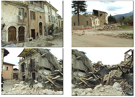
Pictures from Onna town destroyed during the L'Aquila (Abruzzo) earthquake in Italy, April 2009.
On April 6th 2009, at 3:30am, a magnitude 6.3 earthquake struck near the medieval town of L'Aquila, Italy. Almost 300 people died in the tragic event and there were at least 1,500 injured. But besides the humanitarian cost there was also a financial one, as thousands of people were left homeless and many of the city's historical buildings were damaged. In the hours that followed the earthquake, catastrophe modelling companies worked to assess the financial extent of the damage. The resulting loss estimates were not based on on-site surveys or first-hand accounts, but rather on the result of computer models that simulate the effects of natural catastrophes.
But while catastrophe models are indeed used to assess the losses after an event such as the L'Aquila earthquake has occurred, the real task of catastrophe modellers is to provide information concerning the potential for large losses before they occur. The purpose of catastrophe modelling is to anticipate the likelihood and severity of catastrophic events — from earthquakes and hurricanes to terrorism and crop failure — so that companies (and governments) can appropriately prepare for their financial impact.
Our models are applied principally in the insurance market, for example they are used by insurers to assess the potential natural catastrophe loss to property they have insured. Models like ours are helpful in averting bankruptcy of insurers due to overexposure (i.e. too much property in a single area at risk from a single or cluster of events). The models are also helpful in gauging whether the premium charged for insuring a portfolio is sufficient to pay out the insurance claims of home owners and business owners in the event of a catastrophe, based on the magnitude of a loss and its probability of occurrence.
But how do you go about modelling catastrophes? In this article we will focus on the modelling of earthquakes, showing you a skeleton of how catastrophe models work. The models consist of several modules — here we will look at two of them in some detail, the hazard module, which looks at the physical characteristics of potential disasters and their frequency, and the vulnerability module, which assesses the vulnerability (or "damageability") of buildings and their contents when subjected to disasters.
The hazard module
How many earthquakes will there be?
The very first task when trying to estimate potential future losses from a peril is to create a catalogue of events, which is used in modelling. This delivers the baseline data on the earthquakes that may strike, their magnitude, and the likelihood that they will strike.
You may imagine that this catalogue would simply be created from historical and instrumentally recorded events, however this is insufficient for several reasons. Firstly, only significant past events are likely to have been recorded, and they can only have been recorded if someone was there to witness them. This leads to the under-reporting of small events and recording of events only where a population was present, which in turn may lead to underestimating the activity rate of low to moderate magnitude events. What's more, the past is not always indicative of the future: just because something has not happened yet doesn't mean that it will never happen. So using just historical and recently recorded events may lead to vast under-representation of potential losses.
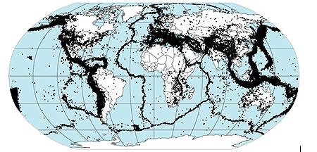
Worldwide recorded events: the characteristics of these events are used to simulate a catalogue of events.
As a solution to this problem, we use statistical and physical models to simulate a large catalogue of events, for example 10,000 scenario years of earthquake experience. Each of the 10,000 years should be thought of as 10,000 potential realisations of what could happen in the year 2010 for example, and not simulations until year 12010. A notional 10,000 year sample is simulated and the collection of the resulting events is called an ensemble. Simulating events in this way gives an accurate picture of the potential risk of events, such as earthquakes, where each scenario year could have no events, one event or multiple events.
Generating theoretical earthquakes
While the event catalogue doesn't consist of events that have actually happened in the past, the models used to generate it do build on historical data on the frequency, location, and magnitude of past earthquakes.
An important tool in this context is the Gutenberg-Richter distribution, which was first developed in the 1930s by Charles Richter and Beno Gutenberg using historical and instrumental data recorded in California. Roughly speaking, the distribution describes how many earthquakes of a given magnitude will occur in a given region during a given time period. The relationship has proved surprisingly robust at each particular seismic source (which can be segments of a fault, or regions in which there is known seismicity, but an undefined fault distribution). Regardless of region and time period, the occurrence pattern of real earthquakes tends to follow the Gutenberg-Richter law.
The Gutenberg-Richter distribution represents a plot of the logarithm (to base 10) of the number of earthquakes $N$, having a magnitude greater than or equal to $M$ plotted against magnitude $M$:
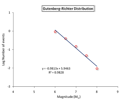
The underlying equation is $$log N = a-bM,$$ where $a$ and $b$ are constants measuring the seismic characteristics of the seismic source in question. In most situations the constant $b$ is equal to 1, so the distribution shows broadly that the number of earthquakes decreases sharply as the magnitude increases, an observation which is intuitively reasonable. For an oversimplified example, by this equation we would expect the number of magnitude 5 earthquakes to be ten times the number of magnitude 6 earthquakes, and 100 times the number of magnitude 7 earthquakes.
We can use the Gutenberg-Richter distribution to say, for example, that if 0.1 earthquakes of magnitude 7.0 are expected in a given region of New Zealand in any year, then we would expect one 7.0 earthquake in a 10 year period (using a time independent view of risk, where the probability that an earthquake occurs does not change with time since the last earthquake). Such information is vital in creating a catalogue that correctly represents the appropriate number of earthquakes of different magnitudes.
The mathematical models that are used to create the catalogue also take into account further information, apart from frequency and magnitude, specifically the characteristics that govern the intensity of earthquake shaking that is felt at different locations. Shaking intensity at the surface depends on such things as the orientation of the fault producing the earthquake, the earthquake's depth, as well as the epicentre of its source. Another important determinant of shaking intensity is soil type. For example, buildings on landfill or soft soils may experience greater ground shaking for the same magnitude event than buildings on solid rock, because such soils can amplify seismic waves.
Ultimately the simulated catalogue of events, when grouped by magnitude and frequency for a specific seismic source, will approximate the Gutenberg-Richter distribution like that shown above, and it will realistically reflect the earthquake pattern one might expect in the given region.
The vulnerability module
What's the damage?
After simulating an event of a given magnitude, the damage it does to buildings must now be computed. Just how badly a particular building will be damaged in an earthquake depends on many factors, but certain characteristics of a building's behaviour serve as a good indicator for the proportion of a building that is likely to be damaged. The cost of the damage is measured by the damage ratio: this is the ratio of the cost to repair a building to the cost of rebuilding it.
The roof drift ratio
A simplistic (though accurate) indicator is the roof drift ratio. The roof drift ratio is the ratio of the displacement $D$ of the roof of a building (relative to the ground) compared to the height of the building $H$, as illustrated in the figure below. Such a measure of displacement is a good proxy for measuring the damage done to the building, as it should be reasonable that the greater the displacement of a building, the more damage is caused during the earthquake's shaking.

The roof drift ratio.
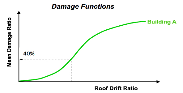
Using laboratory experiments and simulations, as well as statistical data collected from field surveys after real events, it is possible to work out how the roof drift ratio is related to the damage ratio of a building. Nevertheless, it is of course quite possible for seemingly identical buildings, for example buildings with the same roof drift ratio, to experience different levels of damage when impacted by the same intensity of shaking. This is due to small differences in construction and local site specific effects that can have a major impact on losses. To capture this variability of damage, we look not at one definite value for the damage ratio, but at a whole distribution of possible values. The mean of this distribution is known as the mean damage ratio. A graph of the mean damage ratio versus the roof drift ratio is plotted below and is called a vulnerability function. The graph below shows that as the roof drift ratio increases, the mean damage ratio also increases, as expected.
After obtaining the mean damage ratio from the roof drift ratio, we multiply this by the insured value of the building, and now get the expected loss to that building.
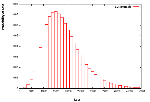
Naively, you can then go on to compute the overall expected insured loss for a particular earthquake by simply adding up the expected losses from all the insured buildings in the region. However, this doesn't account for the variability in buildings' responses to an earthquake of a given strength: for each building there is in fact a distribution of potential losses from the event (see the graph below). This uncertainty is accounted for by a third element, called the financial module, which incorporates specific insurance policy conditions that are pivotal in accurately determining the insurer's loss. The module computes the combined loss distribution of all buildings through a process known as convolution, which is a means of computing all possible combinations of X + Y and their associated probabilities, given the probability distributions of X and Y separately.
The hazard module above gave us a way of assessing how much a particular region is at risk from earthquakes of various magnitudes. The vulnerability and financial modules allow us to compute the loss due to damage from these earthquakes. Putting all these results together gives a reasonably accurate assessment of the losses that are likely to occur in a given region. So while we may not be able to avert disasters, we can at least prepare for their financial impact.
About the author

Shane Latchman works as a Client Services Associate with the catastrophe modelling company AIR Worldwide Limited. Shane works with the earthquake model for Turkey, the hurricane model for offshore assets in the Gulf of Mexico and the testing and quality assurance of the financial module. Shane received his BSc in actuarial science from City University and his Masters in mathematics from the University of Cambridge, where he concentrated on probability and statistics. He also maintains an active role with the Institute of Actuaries.