Non-Euclidean geometry and Indra's pearls
Many people will have seen and been amazed by the beauty and intricacy of fractals like the one shown below. This particular fractal is known as the Apollonian gasket and consists of a complicated arrangement of tangent circles. [Click on the image to see this fractal evolve in a movie created by David Wright.]
Few people know, however, that fractal pictures like this one are intimately related to tilings of what mathematicians call hyperbolic space. One such tiling is shown in figure 1a below. In contrast, figure 1b shows a tiling of the ordinary flat plane. In this article, which first appeared in the Proceedings of the Bridges conference held in London in 2006, we will explore the maths behind these tilings and how they give rise to beautiful fractal images.
 Figure 1a: A non-Euclidean tiling of the disc by regular heptagons. Image created by David Wright. |  Figure 1b: A Euclidean tiling of the plane by regular hexagons. Image created by David Wright. |
Round lines and strange circles
In hyperbolic geometry distances are not measured in the usual way. In the hyperbolic metric the shortest distance between two points is no longer along a straight line, but along a different kind of curve, whose precise nature we'll explore below. The new way of measuring makes things behave in unexpected ways.
As an example, think of a point c and imagine all the points that are a certain distance r away from c. In our ordinary geometry, called Euclidean geometry after the ancient Greek mathematician Euclid, these points form a circle, namely the circle that has centre c and radius r. The circumference of the circle is related to its radius by the well-known equation $$circumference \; = 2 \pi \; \times \; radius.$$

A kale leaf is crinkled up around its edge.
In hyperbolic geometry, because distances are measured differently, the points that are equally far away from our point c still form a circle, but c is no longer at what looks like its centre. The circumference of this hyperbolic circle is proportional not to its radius, but to eradius, where e is the base of the natural logarithm and is roughly equal to 2.718. If the radius is large, then this means that the circumference of a hyperbolic circle is much larger than that of a Euclidean circle. So to fit into ordinary Euclidean space, a big hyperbolic disc has to crinkle up round its edges like a kale leaf. Once you start looking for it, you see this type of growth throughout the natural world. (You can read more about hyperbolic geometry, in the Plus article Strange geometries.)
Hyperbolic tilings in two dimensions ...
The same exponential growth law is manifested in our tiling of figure 1a. Here the disc is filled up by tiles that are arranged in layers around the centre. If you count carefully, you will find that the number of tiles in the nth layer is exactly 7 times the 2nth Fibonacci number:
| Figure 1a |
This is in marked contrast with Euclidean tilings, where the growth law is linear. For example, the honeycomb tiling in figure 1b has exactly 6n hexagons in the nth layer. The numbers here grow much slower:
| Figure 1b |
Despite appearances, in the world of hyperbolic geometry the tiles in figure 1a all have the same size and shape. To fit the tiles into a Euclidean picture, we have to shrink their apparent size as we move away from the centre of the disc, so that to our Euclidean glasses the tiles look smaller and smaller as they pile up near the edge of the disc. Since you can fit infinitely many layers of tiles between the centre of the disc and its boundary, in our hyperbolic way of measuring, the boundary must be infinitely far away from the centre. In this strange geometry the diameter of the disc is infinite. For this reason, the boundary circle is called the circle at infinity.
Figure 2: All of the hyperbolic plane fits into the disc bounded by the blue circle. The role of straight lines in this geometry is played by arcs of circles that meet the boundary in right angles, like the red arc shown here.
Measured in the hyperbolic metric, the sides of each tile in figure 1a have the same length, as do the sides of any two distinct tiles. Although the sides of each tile look slightly curved to us, in the hyperbolic metric they are actually straight. To understand this, forget about your intuitive understanding of straightness for a moment and take a slightly more abstract view: a path is "straight" if it gives you the shortest distance between its end-points. In the hyperbolic metric, the shortest distance between two points is along the arc of a circle that meets the circle at infinity at right angles, as shown in figure 2. The sides of the tiles in figure 1a are pieces of circles with precisely this property. The tiles are bounded by straight line segments all of which have the same length and, as it turns out, meet at the same angle — the tiles are regular hyperbolic polygons.
If you were a two-dimensional hyperbolic being, the tiles shown in figure 1a would all seem the same to you, they would all look like regular heptagons. Since the boundary circle is infinitely far away, you would never be able to get to it or even be aware of it. Your whole world would be contained inside the disc, with the tiles stretching out to the horizon like an infinite chess board.
... and in three dimensions
Figure 3: A cube is a volume enclosed by six intersecting planes. Each of the six faces of the cube is part of one of these planes.
Now imagine a similar geometry in three dimensions. Just as the two-dimensional hyperbolic plane can be visualised as a disc enclosed by its circle at infinity, so the three-dimensional hyperbolic universe can be visualised as a solid ball, enclosed in a Euclidean sphere. The sphere's boundary is infinitely far, in hyperbolic terms, away from its centre.
The tiles now become solid three-dimensional objects, the hyperbolic analogue of polyhedra. In Euclidean geometry regular polyhedra are volumes enclosed by a number of intersecting flat planes. A cube, for example, is the volume you get from six planes, each intersecting four others at right angles (see figure 3).
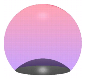
Figure 4: Hyperbolic 3-space can be visualised as the inside of a sphere. A hyperbolic plane is a part of a plane that meets the sphere at infinity at right angles. Image created by David Wright.
But what does a hyperbolic plane look like? In two-dimensional hyperbolic space the role of straight lines was played by circular arcs meeting the bounding circle at right angles. Similarly, the role of planes in hyperbolic three-space is played by pieces of spheres. These sit inside the big sphere that bounds our hyperbolic universe, meeting the boundary sphere at right angles (see figure 4).
A hyperbolic polyhedron is the volume you get by intersecting several hyperbolic planes. And just as you can tile Euclidean space by certain polyhedra, for example by cubes, you can tile hyperbolic three-space by hyperbolic polyhedra. Figure 5, a still from the remarkable movie Not Knot!, shows such a tiling seen from deep inside hyperbolic space, far away from the bounding sphere at infinity.
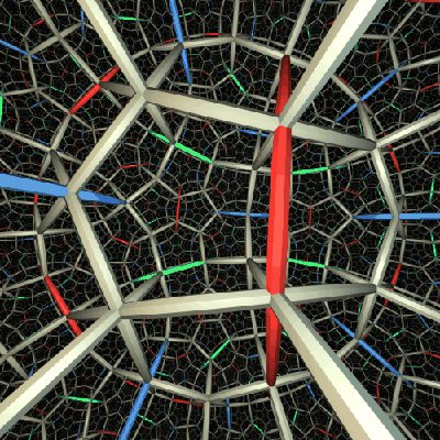
Figure 5: A tiling of three-dimensional hyperbolic space. Image created by Charles Gunn of the Technische Universität Berlin. It is a still from the movie Not Knot!, published by A K Peters Ltd.
The window pane at infinity
As you might imagine from figure 5, tilings of hyperbolic 3-space are rather hard to draw. As an easier substitute, mathematicians usually study what they see on the boundary of hyperbolic space, that is on the sphere that defines the hyperbolic universe. The patterns we get here are of amazing beauty. They are easier to describe because the surface of a sphere is a two-dimensional object and can be projected onto a flat plane.
In two dimensions the analogue of this would be to study what we can see on the boundary of the disc, namely the circle. In the case of figure 1a this is not very interesting: the tiles simply pile up all the way round the circle. Now suppose that the original tile is still a polygon with a finite number of sides, but that it stretches all the way out to the boundary, like the yellow region in figure 6. Then each of its copies meets the circle in four circular arcs. Although the tiles fill up all of two-dimensional hyperbolic space (the interior of the disc), the totality of the arcs do not fill up the whole circle.
Figure 6: A non-Euclidean tiling of the disc by a polygon with some sides at infinity. Image created by David Wright.
The set of omitted points has interesting properties, for example it is a fractal. It is an example of what is called mathematically a Cantor set, more colloquially, a fractal dust. (You can find out more about Cantor sets in Plus articles Measure for measure and How big is the Milky Way?)
If you were a two-dimensional being living in the same plane as the disc, but outside it, then what you would see of each hyperbolic polygon would be the circular arc in which it meets the boundary circle. In three dimensions the analogue of a polygon with a finite number of sides is a polyhedron with a finite number of faces. Outside observers will see these faces as shadows where the polyhedron meets the sphere. Figure 7a below shows the sphere with four-sided shapes which are faces of polyhedra that tile its inside. They pile up in remarkable patterns on the boundary of the sphere, like noses pressed against a window pane. Figure 7b shows the patterns on the sphere projected onto the plane; this time with a different colour scheme.
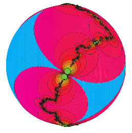 Figure 7a: Faces of polyhedra in a 3-dimensional hyperbolic tiling pressed against the sphere at infinity. Image created by David Wright. | 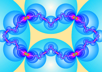 Figure 7b: The tiling of the sphere projected onto the plane. Image created by David Wright. |
Patterns like this were studied by the German mathematician Felix Klein (1849 - 1925). In the 1980s David Mumford realised that they were a natural target for computer exploration. With David Wright, he embarked on a systematic study which eventually resulted not only in inspiring new mathematics, but also in the book Indra's Pearls.
The book shows off some of the remarkable patterns that arise on the window pane at infinity. It explains these patterns with the minimum of mathematical baggage, but with enough detail for the mathematically inclined to follow the reasoning and for the computationally inclined to make their own pictures.
The maths
The Euclidean tiling from Figure 1 again.
To create a two-dimensional tiling, whether it's Euclidean like the one of figure 1b, or hyperbolic, you need a way of creating identical copies of an initial tile and placing them alongside each other. Mathematically, this job is done by reflections, rotations and translations: you get to each tile either by shifting your initial tile into a given direction by a given distance — this is known as a translation — by reflecting it in an axis, or by rotating it through a given angle around a fixed point. Or, indeed, by a combination of any of these three movements.
Rotations, reflections and translations, and the movements you get by doing them in sequence, are collectively known as rigid motions or symmetries. "Rigid" because they do not distort distances or angles and "symmetries" because they can leave symmetrical shapes unchanged.
To describe a tiling, all you need is a description of the initial tile together with a list of symmetries that generate the tiling. Although there are infinitely many tiles, the list of symmetries can be finite, because it may be possible to get to all the tiles by performing the same symmetries over and over again.
The same is true of three-dimensional Euclidean space. To tile it by polyhedra, for example by cubes, you start with a central polyhedron and repeatedly perform a number of symmetries, only this time you allow three-dimensional rotations, translations and reflections.
Tilings of three-dimensional hyperbolic space are generated in the same way: you start with a hyperbolic polyhedron and repeatedly perform a number of hyperbolic symmetries until you have filled up the whole universe. Without thinking too hard about what hyperbolic symmetries might look like, remember that we are interested in what happens on the sphere that bounds our hyperbolic universe. This means that we need to start with a face of the polyhedron that presses against the bounding sphere and repeatedly perform a number of movements, watching copies of the face pile up on the sphere as they do in figure 7.
But how can we describe these movements? Remember that our symmetries leave hyperbolic distance intact. But we are working on the bounding sphere at infinity, where we can no longer measure distance in the same way. In fact, on the window pane at infinity it is impossible to find a way of measuring distance that is preserved. But all is not lost: it turns out that the transformations we are looking for do leave something intact. They transform circles into circles, with changes of radius being allowed. Such transformations are called Möbius transformations, after the German mathematician August Möbius (1790 - 1868).
To describe these transformations, mathematicians project the sphere onto a flat plane using stereographic projection: place a light bulb on the North pole of the sphere so that each point of the sphere has its unique and very own shadow on the plane below. Every point except the North pole that is, but mathematicians have a way of dealing with this and we can safely ignore the North pole here.
Figure 8: Stereographic projection - draw a line from the North pole through a given point on the sphere. The point's shadow is the place where the line hits the plane below. Image created by David Wright.
The formulae of Möbius transformations look neatest when we use complex numbers. If we think of each point (x,y) of the plane as the corresponding complex number z = x + iy, then a Möbius transformations transforms the plane by moving each point z to
$$ \frac{az+b}{cz+d},$$
where a, b, c and d are fixed complex numbers. (If you'd like to find out more about complex numbers, read this short introduction or the Plus article Curious quaternions.)
Piling up
What we really want to study is how tiles like those in figure 7 (or, more precisely, their projected images in the plane) pile up in the plane as they are being moved around by Möbius transformations. For example, we can start with the two transformations $$ z \to \frac{1}{-2iz+1} \;\;\;\; and \;\;\;\; z \to \frac{(1-i)z+1}{z+1+i}.$$ Then take a basic shape, say a stick man, and apply both of these transformations to the figure over and over again. As you can see in figure 9, the images get small and are distorted as the level of the repetition increases. If you choose the starting transformations cleverly, the patterns which emerge when the images pile up are amazingly beautiful.
Figure 9: Images of a man under repeated applications of Möbius transformations. Movie created by David Wright.
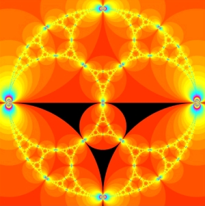
To see more clearly what is going on, we often drop the original shape altogether and just look at the region where its smaller and smaller images pile up. This is called the limit set or chaotic set of the iteration, because in this part of the pictures the symmetries act in a chaotic way. (Though to a mathematician, the chaos is very controlled.) The limit set is shown in figure 10.
 Figure 10: The limit set. |
By choosing the initial symmetries with enough care, we can create limit sets with intricate patterns of tangent circles. The two transformations written down above produce the famous Apollonian Gasket, which is shown at the beginning of this article.
In other examples the tangent circles spiral in beautiful patterns:
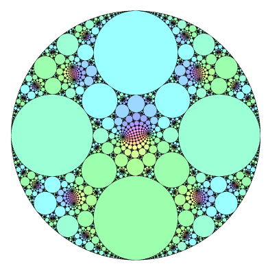
Figure 11: Another limit set. Image created by David Wright.
A similar spiralling pattern is shown below. After drawing the limit set, the program will zoom in on it, revealing the breathtaking intricacy of this fractal. The movie was created by David Wright
How and why these beautiful fractals arise from the maths is explored in great detail in the book and its accompanying website, which also contains instructions for programming your own images.
Indra's pearls
Why did we call our book Indra's Pearls? In western thought, the infinite is conceived as counting without end, a flock of sheep going through the gate forever: one, two, three, .. one hundred and one, one hundred and two, ..... But there are other ways of getting to infinity. Remember the man with seven wives. Kits, cats, sacks and wives, quite a lot of traffic enroute to St Ives! In fact the traffic increases exponentially with the number of levels (kits, cats,...).
Such exponential growth reminds us of hyperbolic tilings, typically formed by a similar repetitive process. In figure 13 below, we start with six disjoint circles. For each circle C it is possible to find a transformation which swaps the inside and the outside of C and leaves every point on C itself fixed. These transformations are often called inversions — inverting in C is reminiscent of a "reflection", only we don't reflect in a straight line, but in the circle. Except for the fact that, like any reflection, it turns things back to front, an inversion is a special kind of Möbius transformation. When we perform this "reflection" in C, the other five circles, which are outside C, get reflected into five smaller circles inside it. If we do this for each of the six circles, we end up with each of them containing five smaller second level circles. The repeat operation produces five more small circles inside each of these second level circles: now each of the six initial circles contains 52 = 25 circles in all. At the next level, we will have 53 = 125 tiny circles. And so on.
Figure 13: Worlds within worlds. Image created by David Wright.
In many eastern philosophies, especially Buddhist, this idea of the infinite appearing from copies within copies is pervasive: "In a single atom, great and small lands, as many as atoms." This concept was so exactly reflected in the mathematics of our pictures that it inspired our title, taken from the ancient Buddhist myth of Indra's Web:
In the heaven of the great god Indra is said to be a vast and shimmering net, finer than a spider's web, stretching to the outermost reaches of space. Strung at each intersection of its diaphanous threads is a reflecting pearl. Since the net is infinite in extent, the pearls are infinite in number. In the glistening surface of each pearl are reflected all the other pearls, even those in the furthest corners of the heavens. In each reflection, again are reflected all the infinitely many other pearls, so that by this process, reflections of reflections continue without end.
About this article
A version of this article first appeared in the Bridges (Mathematical Connections in Art Science and Music) Conference Proceedings held in 2006 in London. Copies of the Proceedings can be obtained from Tarquin Books in Europe and at mathartfun.com in the US.
The book Indra's Pearls was written by David Mumford, Caroline Series and David Wright. It is published by Cambridge University Press.

Caroline Series is a Professor of Mathematics at Warwick University. She was born and educated in Oxford and was an undergraduate at Somerville. Having done her PhD at Harvard as a Kennedy scholar, she returned to the UK and has been at Warwick since 1979. She likes finding the patterns behind geometrical structures, and her research area, non-Euclidean or hyperbolic geometry, is closely related to fractals and chaos.
David Wright gained his doctorate in number theory in 1982 from Harvard under the excellent direction of Barry Mazur, despite spending most of his time engaged in visual mathematical explorations with David Mumford. He is currently Professor of Mathematics at Oklahoma State University, and has two wonderful daughters Alexandra and Julie. The author's picture was provided by the latter, currently a concentrator in Visual Arts, French and Mathematics at Harvard.
Comments
Anonymous
These non-Euclidean shapes are beautiful.
I can see why my husband liked Maths so much that he studied it for all those years at Open Uni! It is so interesting.
Sunny H. from NZ
Anonymous
I thought you might be interested to see this three dimensional model of tessellated heptagons based on the two dimensional model in the article.
http://images4-d.ravelrycache.com/uploads/michaela112358/249770763/IMG_…
Dianne
David, Thank you so much for this beautiful, inspiring work!