Think drug-induced hallucinations, and the whirly, spirally, tunnel-vision-like patterns of psychedelic imagery immediately spring to mind. But it's not just hallucinogenic drugs like LSD, cannabis or mescaline that conjure up these geometric structures. People have reported seeing them in near-death experiences, as a result of disorders like epilepsy and schizophrenia, following sensory deprivation, or even just after applying pressure to the eyeballs. So common are these geometric hallucinations, that in the last century scientists began asking themselves if they couldn't tell us something fundamental about how our brains are wired up. And it seems that they can.

Computer generated representations of form constants. The top two images represent a funnel and a spiral as seen after taking LSD, the bottom left image is a honeycomb generated by marijuana, and the bottom right image is a cobweb. Image from [1], used by permission.

Geometric hallucinations were first studied systematically in the 1920s by the German-American psychologist Heinrich Klüver. Klüver's interest in visual perception had led him to experiment with peyote, that cactus made famous by Carlos Castaneda, whose psychoactive ingredient mescaline played an important role in the shamanistic rituals of many central American tribes. Mescaline was well-known for inducing striking visual hallucinations. Popping peyote buttons with his assistant in the laboratory, Klüver noticed the repeating geometric shapes in mescaline-induced hallucinations and classified them into four types, which he called form constants: tunnels and funnels, spirals, lattices including honeycombs and triangles, and cobwebs.

In the 1970s the mathematicians Jack D. Cowan and G. Bard Ermentrout used Klüver's classification to build a theory describing what is going on in our brain when it tricks us into believing that we are seeing geometric patterns. Their theory has since been elaborated by other scientists, including Paul Bressloff, Professor of Mathematical and Computational Neuroscience at the newly established Oxford Centre for Collaborative Applied Mathematics.

How the cortex got its stripes...

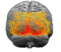
The visual cortex: the area V1 is shown in red. Image: Washington irving

In humans and mammals the first area of the visual cortex to process visual information is known as V1. Experimental evidence, for example from fMRI scans, suggests that Klüver's patterns, too, originate largely in V1, rather than later on in the visual system. Like the rest of the brain, V1 has a complex, crinkly, folded-up structure, but there's a surprisingly straight-forward way of translating what we see in our visual field to neural activity in V1. "If you imagine unfolding [V1]," says Bressloff, "You can think of it as neural tissue a few millimetres thick with various layers of neurons. To a first approximation, the neurons through the depth of the cortex behave in a similar way, so if you compress those neurons together, you can think of V1 as a two-dimensional sheet."

From the visual field to the visual cortex

Think of the visual field as a flat sheet, endowed with polar coordinates: each point in the field is defined by two numbers , where is its distance to the origin , and the angle between the line and the -axis. The origin corresponds to the centre of the visual field. V1 is also modelled as a flat sheet, this time endowed with the usual Cartesian coordinates . The exact coordinate map between the visual field and the flat model of V1 is complicated to write down, but for points in the visual field that are away from the centre of the field (so for sufficiently large) it is similar to the logarithmic map

This map transforms a circle of radius in the visual field into a vertical straight line segment at , and a ray emanating from the origin at angle into a horizontal straight line segment at .

An object or scene in the visual world is projected as a two-dimensional image on the retina of each eye, so what we see can also be treated as flat sheet: the visual field. Every point on this sheet can be pin-pointed by two coordinates, just like a point on a map, or a point on the flat model of V1. The alternating regions of light and dark that make up a geometric hallucination are caused by alternating regions of high and low neural activity in V1 — regions where the neurons are firing very rapidly and regions where they are not firing rapidly.

To translate visual patterns to neural activity, what is needed is a coordinate map, a rule which links each point in the visual field to a point on the flat model of V1. In the 1970s scientists including Cowan came up with just such a map, based on anatomical knowledge of how neurons in the retina communicate with neurons in V1 (see the box on the right for more detail). For each light or dark region in the visual field, the map identifies a region of high or low neural activity in V1.

So how does this retino-cortical map transform Klüver's geometric patterns? It turns out that hallucinations comprising spirals, circles, and rays that emanate from the centre correspond to stripes of neural activity in V1 that are inclined at given angles. Lattices like honeycombs or chequer-boards correspond to hexagonal activity patterns in V1. This in itself might not have appeared particularly exciting, but there was a precedent: stripes and hexagons are exactly what scientists had seen when modelling other instances of pattern formation, for example convection in fluids, or, more strikingly, the emergence of spots and stripes in animal coats. The mathematics that drives this pattern formation was well known, and it now suggested a mechanism for modelling the workings of the visual cortex too.

...and how the leopard got its spots

The first model of pattern formation in animal coats goes back to Alan Turing, better known as the father of modern computer science and Bletchley Park code breaker. Turing was interested in how a spatially homogeneous system, such as a uniform ball of cells making up an animal embryo, can generate a spatially inhomogeneous but static pattern, such as the stripes of a zebra.

Animal pattern equations

For the sake of simplicity, imagine the embryo as a one-dimensional line. At any time and any point on the embryo, the concentrations of the activator and inhibitor are given by the functions and respectively. These functions vary over time according to the following rules:

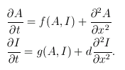
The first term on the right-hand side of each equation describes how much activator/inhibitor is being produced. These terms are functions of activator and inhibitor concentrations because they both affect the reaction rate.

The second term in each equation is a second derivative describing how quickly the gradient of activator/inhibitor is changing. These terms give the rate of diffusion.

The extra term, d, on the right-hand side of the second equation is the diffusion coefficient — how much quicker the inhibitor diffuses than the activator. The inhibitor being a faster diffuser was shown by Turing to be pivotal in driving the process of pattern generation.

Turing hypothesised that these animal patterns are a result of a reaction-diffusion process. Imagine an animal embryo which has two chemicals living in its skin. One of the two chemicals is an inhibitor, which suppresses the production of both itself and the other chemical. The other, an activator, promotes the production of both.

Initially, at time zero in Turing's model, the two chemicals exactly balance each other — they are in equilibrium, and their concentrations at the various points on the embryo do not change over time. But now imagine that, for some reason or other, the concentration of activator increases slightly at one point. This small perturbation sets the system into action. The higher local concentration of activator means that more activator and inhibitor are produced there — this is a reaction. But both chemicals also diffuse through the embryo skin, inhibiting or activating production elsewhere.

For example, if the inhibitor diffuses faster than the activator, then it quickly spreads around the point of perturbation and decreases the concentration of activator there. So you end up with a region of high activator concentration bordered by high inhibitor concentration — in other words, you have a spot of activator on a background of inhibitor. Depending on the rates at which the two chemicals diffuse, it is possible that such a spotty pattern arises all over the skin of the embryo, and eventually stabilises. If the activator also promotes the generation of a pigment in the skin of the animal, then this pattern can be made visible. (See the Plus article How the leopard got its spots for more detail.)

Turing wrote down a set of differential equations which describe the competition between the two chemicals (see the box on the right), and which you can let evolve over time, to see if any patterns emerge. The equations depend on parameters capturing the rate at which the two chemicals diffuse: if you choose them correctly, the system will eventually stabilise on a particular pattern, and you can vary the pattern by varying the parameters. Here is an applet (kindly provided by Chris Jennings) which allows you to play with different parameters and see the patterns form.

Patterns in the brain

Neural activity in the brain isn't a reaction-diffusion process, but there are analogies to Turing's model. "Neurons send signals to each other via their output lines called axons," says Bressloff. Neurons respond to each other's signals, so we have a reaction. "[The signals] propagate so quickly relative to the process of pattern formation, that you can think of them as instantaneous interactions." So rather than diffusion, which is a local process, we have instantaneous interaction at a distance in this case. The roles of activator and inhibitor are played by two different classes of neurons. "There are neurons which are excitatory — they make other neurons more likely to become active — and there are inhibitory neurons, which make other neurons less likely to become active," says Bressloff. "The competition between the two classes of neurons is the analogue of the activator-inhibitor mechanism in Turing's model."

Stripy, hexagonal and square patterns of neural activity in V1 generated by a mathematical model. Image from [1], used by permission.

Inspired by the analogies to Turing's process, Cowan and Ermentrout constructed a model of neural activity in V1, using a set of equations that had been formulated by Cowan and Hugh Wilson. Although the equations are more complicated than Turing's, you can still play the same game, letting the system evolve over time and see if patterns in neural activity evolve. "You find that, under certain circumstances, if you turn up a parameter which represents, for example, the effect of a drug on the cortex, then this leads to a growth of periodic patterns," says Bressloff.

Cowan and Ermentrout's model suggests that geometric hallucinations are a result of an instability in V1: something, for example the presence of a drug, throws the neural network off its equilibrium, kicking into action a snowballing interaction between excitatory and inhibitory neurons, which then stabilises in a stripy or hexagonal pattern of neural activity in V1. In the visual field we then "see" this pattern in the shape of the geometric structures described by Klüver.

Symmetries in the brain

In reality, things aren't quite as simple as in Cowan and Ermentrout's model, because neurons don't only respond to light and dark images. Through the thickness of V1, neurons are arranged in collections of columns, known as hypercolumns, with each hypercolumn roughly responding to a small region of the visual field. But the neurons in a hypercolumn aren't all the same: apart from detecting light and dark regions, each neuron specialises in detecting local edges — the separation lines between light and dark regions in a part of an image — of a particular orientation. Some detect horizontal edges, others detect vertical edges, others edges that are inclined at a 45° angle, and so on. Each hypercolumn contains columns of neurons of all orientation preferences, so that a hypercolumn can respond to edges of all orientations from a particular region of the visual field. It is the lay-out of hypercolumns and orientation preferences that enables us to detect contours, surfaces and textures in the visual world.

Connections in V1: Neurons interact with most other neurons within a hypercolumn. But they only interact with neurons in other hypercolumns, if the columns lie in the direction of their orientation, and if the neurons have the same preference. Image from [2], used by permission.

Over recent years, much anatomical evidence has accumulated showing just how neurons with various orientation preferences interact. Within their own hypercolumn, neurons tend to interact with most other neurons, regardless of their orientation preference. But when it comes to neurons in other hypercolumns they are more selective, only interacting with those of similar orientations and in a way which ensures that we can detect continuous contours in the visual world.

Bressloff, in collaboration with Cowan, the mathematician Martin Golubitsky and others, has generalised Cowan and Ermentrout's original model to take account of this new anatomical evidence. They again used the plane as the basis for a model of V1: each hypercolumn is represented by a point on the plane, while each point in turn corresponds to a hypercolumn. Neurons with a given orientation preference (where is an angle between 0 and ) are represented by the location of the hypercolumn they're in, together with the angle , that is, they are represented by three bits of information, . So in this model V1 is not just a plane, but a plane together with a full set of orientations for each point.

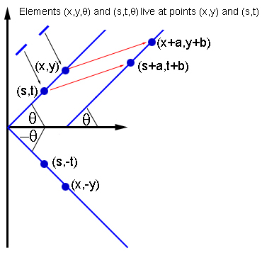
If two elements (x,y,θ) and (s,t,θ) interact, then so do the elements of the same orientation at (x+a,y+b) and (s+a,t+b), and the elements of orientation -θ at (x,-y) and (s,-t).

In keeping with anatomical evidence, Bressloff and his colleagues assumed that a neuron represented by interacts with all other neurons in the same hypercolumn But it only interacts with neurons in other hypercolumns, if these hypercolumns lie in their preferred direction : on the plane, draw a line through of inclination Then the neurons represented by interact only with neurons in hypercolumns that lie on this line, and which have the same preferred orientation .

This interaction pattern is highly symmetric. For example, the pattern doesn't appear any different if you shift the plane along in a given direction by a given distance: if two elements and interact, then the elements you get to by shifting along, that is and for some and , interact in the same way. In a similar way, the pattern is also invariant under rotations and reflections of the plane.

A lattice tunnel hallucination generated by the mathematical model. It strongly resembles hallucinations seen after taking marijuana. Image from [1], used by permission.

Bressloff and his colleagues used a generalised version of the equations from the original model to let the system evolve. The result was a model that is not only more accurate in terms of the anatomy of V1, but can also generate geometric patterns in the visual field that the original model was unable to produce. These include lattice tunnels, honeycombs and cobwebs that are better characterised in terms of the orientation of contours within them, than in terms of contrasting regions of light and dark.

What's more, the model is sensitive to the symmetries in the interaction patterns between neurons: the mathematics shows that it is these symmetries that drive the formation of periodic patterns of neural activity. So the model suggests that it is the lay-out of hypercolumns and orientation preferences, in other words the mechanisms that enable us to detect edges, contours, surfaces and textures in the visual world, that generate the hallucinations. It is when these mechanism become unstable, for example due to the influence of a drug, that patterns of neural activity arise, which in turn translate to the visual hallucinations.

Beyond hallucinations

Bressloff's model does not only provide insight into the mechanisms that drive visual hallucinations, but also gives clues about brain architecture in a wider sense. In collaboration with his wife, an experimental neuroscientist, Bressloff has looked at the connection circuits between hypercolumns in normal vision, to see how visual images are processed. "People used to think that neurons in V1 just detect local edges, and that you have to go to higher levels in the brain to put these edges together to detect more complicated features like contours and surfaces. But the work I have done with my wife shows that these structures in V1 actually allow the earlier visual cortex to detect contours and do more global processing. It used to be thought that you process more and more complex aspects of an image as you go higher up in the brain. But now it's realised that there is a huge amount of feedback between higher and lower cortical areas. It's not a simple hierarchical process, but an incredibly complicated and active system it will take many years to understand."

Practical applications of this work include computer vision — computer scientists are already building the inter-connectivity structures that Bressloff and his colleagues played around with into their models, with the aim of teaching computers to detect contours and textures. On a more speculative note, Bressloff's research may also one day help to restore vision to visually impaired people. "The question here is if you can somehow stimulate part of the visual cortex, [bypassing the eye], and use that to guide a blind person," says Bressloff. "If one can understand how the cortex is wired up and responds to stimulation, perhaps one would then have a better way of stimulating it in the right way."

There are even applications that have nothing at all to do with the brain. Bressloff applied the insights from this work to other situations in which objects are located in space and also have an orientation, for example fibroblast cells found in human and animal tissue. He showed that under certain circumstances these interacting cells and molecules can line up and form patterns analogous to those that arise in V1.

People have reported seeing visual hallucinations since the dawn of time and in almost all human cultures — hallucinatory images have even been found in petroglyphs and cave paintings. In shamanistic traditions around the world they have been regarded as messages from the spirit world. Few neuroscientists today would agree that spirits have anything to do with it, but as messengers from a hidden world — this time the hidden world of our brain — these hallucinations seem to have lost none of their potency.

Further reading

Bressloff's work on visual hallucinations is summarised in the paper What geometric visual hallucinations tell us about the visual cortex ([1]). A more detailed description can be found in the paper Geometric visual hallucinations, Euclidean symmetry and the functional architecture of striate cortex ([2]).

About this article

Paul Bressloff was interviewed by Marianne Freiberger, co-editor of Plus, in August 2009.

Paul Bressloff graduated with a degree in physics from Oxford 1981 and completed a PhD in string theory at King's College London in 1988. He then spent five years as a research Scientist at GEC-Marconi Hirst Research Centre, where he worked on dynamical systems theory and neural networks. In 1993 he joined the Department of Mathematical Sciences at Loughborough University, where he built up a group in mathematical biology and became Professor of Applied Mathematics in 1998. Tenured Full Professor at the University of Utah he built up a group in mathematical neuroscience between 2001 and 2009. He returned to the UK in July 2009 to take up an appointment as a University Research Professor in Mathematical Neuroscience at the University of Oxford. He has also been awarded a Royal Society Wolfson Merit Award (2009-2014).

Bressloff has spent the past 20 years working at the multidisciplinary interface between applied mathematics, theoretical physics and neuroscience. The main focus of his work is to understand how the brain functions as a complex dynamical system at multiple spatial and temporal scales in healthy and diseased brains. He has published more than 120 papers in research journals and co-authored one book. He has mentored ten PhD students and four postdocs.