See here for the first part of this article.

Shifty dynamics continued

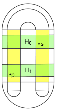
The point p is the fixed point with a sequence consisting of all 1s. The point s is the the fixed point with a sequence consisting of all 0s.

Translating the dynamics of to the dynamics of shifting a dot around bi-infinite sequences immediately tells us that the horseshoe map has two fixed points, which stay exactly where they are when you apply to them. These are the points and corresponding to the sequences

and

respectively. The two sequences remain the same as you shift the dot to the left or right.

There are also two points of period 2: these are points that are mapped by to another point , which in turn maps back to . The period 2 points have the sequences

and

These two sequences remain the same as you shift the dot to the left or right by two places. And as you can easily see, they corresponding points map to each other under .

Similarly, there are also period 3 points (we’ll leave it up to you to find the corresponding sequences), and in fact points of any period . This, for example, is the sequence representing a point with period .

In fact, it turns out that periodic points are everywhere. Given any bi-infinite sequence with a dot, you can always construct a periodic sequence that agrees with it to as many places as you like (to the left and right of the dot). Simply take a chunk containing the dot in the middle and repeat it to the left and right. For example, given the sequence

(with only to the left and only s to the right of the dot) consider the periodic sequence

It agrees with the original sequence in three places to the left and right of the point. This means the corresponding points in are close to each other. The fact that the second sequence is periodic (repeating after six shifts of the dot) means that the point corresponding to it is a periodic point of period six.

You can construct a periodic sequence that agrees with the original one to as many places as you like, not just six. This implies that arbitrarily close to any point in there’s a periodic point. (Technically, periodic points are dense in

The butterfly effect

The butterfly effect got its name from the idea that the bat of a butterfly's wing in one place on the Earth can cause a tornado elsewhere. That's sensitive dependence on initial conditions.

All this periodicity doesn’t mean that horseshoe map behaves in a nice and predictable fashion - far from it!

Imagine I stab my pencil at a point in and ask you to compute its forward orbit. Now the tip of my pencil isn’t infinitely sharp, so you don’t really know exactly where is. But surely a good approximation should be good enough to give us a good approximation of its forward orbit?

It isn’t. In the tiny region located by my pencil’s tip there’ll be all sorts of points in , each of which you could use for your approximation. Their sequences will agree to a large number of places because they are all very close together. However, there will always be a place where two sequences don’t agree: where one has a while the other has a . Now look at the forward orbits of the two corresponding points. Applying means shifting the dot to the right by one place in each sequence. As you apply again and again, the parts of the sequences that agree get eaten up, until one sequence has a right after the dot and the other has a . This means that one of the corresponding points is in and the other in .

As an example, consider the fixed point

and the point

These two are close, but after applying seven times we end up with the points

and

The first of these lies in and the second in . This is pretty much as far away as two points in can be. Our small initial imprecision has snowballed into a large difference.

This sensitive dependence on initial conditions occurs in other dynamical systems too. It is one of the reasons why we can’t predict the weather or the stock market with high degrees of accuracy: we can never get initial conditions 100% right, so long-term predictions are likely to turn out wrong. The phenomenon is also known as the butterfly effect.

Messing around with sequences you can also show quite easily that any neighbourhood of near-by points in , under repeated application of , will eventually overlap any other neighbourhood of points in . The map truly mixes things up — and this property is appropriately called topological mixing.

The three properties we have found using our sequences, the density of periodic orbits, sensitive dependence on initial conditions and topological mixing, are considered the hall marks of mathematical chaos. They mean that things go wild and unpredictable as you apply repeatedly. The horseshoe map, so simple at first sight, is a beautiful example of chaos.

Poincaré

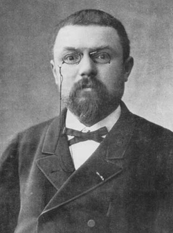
Henri Poincaré. He was shocked by his discovery of homoclinic tangles.

What does all this have to do with the mess Poincaré found himself in 1889? In 1960 Stephen Smale (building on work by David Birkhoff) proved that the horseshoe is in some sense universal. A large class of dynamical systems, defined by mathematical equations, contain the dynamics of the horseshoe map and therefore also contain its chaos.

Everything hinges on the existence of a particular point. In the case of the horseshoe map, an example is the point with the sequence with only s at the left and right end. Points in the forward orbit of get closer and closer to the fixed point , whose sequence consists entirely of s. That's a result of the fact that squeezes things in the horizontal direction: itself might be far away from , but as you apply things get squeezed so the forward orbit of moves closer to . The backward orbit of also gets closer and closer to — that's a result of the fact that stretches things in the vertical direction (if stretches things, then run backwards squeezes them). The existence of the point somehow embodies the squeezing and the stretching of , whose interaction appears to be behind the chaos. The point is called a homoclinic point of .

Loosely speaking, if a dynamical system has such a homoclinic point, which behaves just like does for the horseshoe map, then the dynamical system contains the full dynamics of the horseshoe map. (This is a very loose formulation of Smale's theorem. For a more technical version, see here.)

The dynamical systems Poincaré considered when thinking about the three-body system can contain such homoclinic points. The mess that results from the dynamics is called a homoclinic tangle and trying to draw it is a bit like trying to draw the forward and backward orbits of our region , which include all those multi-folded horseshoes. As Poincaré wrote:

There's another interesting connection between Smale and Poincaré we should mention. Poincaré made an important conjecture, not in the area of dynamical systems, but in the area of topology. The conjecture now bears Poincaré's name, and wasn't proved until the early 2000s. In 1961 however, Smale proved a result very much related to the Poincaré conjecture (he proved it for dimensions greater than 5). Rather satisfyingly his prove made use of dynamical techniques. It earned him the 1966 Fields Medal, one of the highest honours in maths.

About this article

Marianne Freiberger is editor of Plus. She talked to Stephen Smale at the Heidelberg Laureate forum 2017.