Reconstructing the tree of life
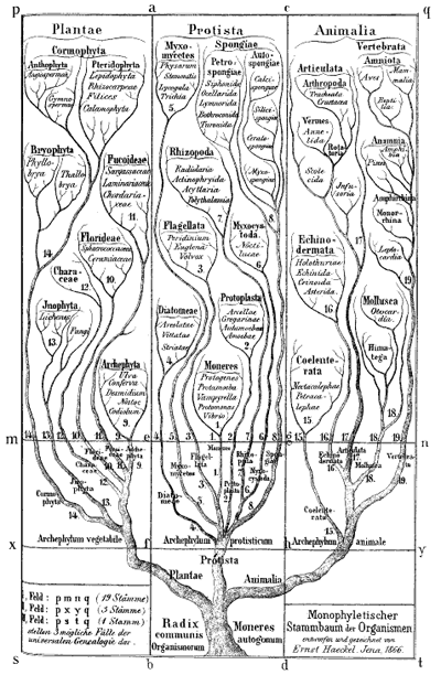
Ernst Haeckel's Monophyletic tree of organisms, 1866. Biologists at the time identified three major groups of species: animals, plants and protista; primitive, mostly unicellular, organisms. Modern biologists also classify all life into three groups, but now animals and plants are considered to belong to the same group, with two different types of bacteria making up the other two groups.
Next year is a great one for biology: not only will we celebrate 150 years since the publication of On the origin of species, but also 200 years since the birth of its author, Charles Darwin. And two important anniversaries these are indeed: Darwin's theory of evolution through natural selection revolutionised vast swathes of human thought, from hard science to religion. Recent advances in genetics have lent a whole new dimension to Darwin's basic tenet, and furnished it with a vast body of evidence.
Mathematics has remained largely untouched by this revolution. Biology and mathematics have been relatively separate disciplines throughout their long histories, in stark contrast to the rampant cross-fertilisation between mathematics and physics. But this may be about to change. As scientists develop faster methods for sequencing genes and whole genomes, genetics is experiencing an information explosion. Mathematical methods are needed to tame huge amounts of data, and to infer from them the true underlying path of evolution.
But it's not all about quantity. At the heart of evolution lies a beautifully simple mathematical object: the evolutionary tree. The quest to understand it has spawned recent collaborations between mathematicians and biologists and thrown up simple mathematical questions that look like they should have been answered centuries ago. In this article we look at a few of these.
The tree of life
The central assumption of phylogenetics, the study of genetic relationships, is that all life on Earth stems from a single common ancestor. As individuals procreate, genes mutate, probably randomly, and beneficial mutations are passed on through natural selection. Groups of individuals change, adapting to their environment, until eventually they become reproductively isolated and form a new species of their own.
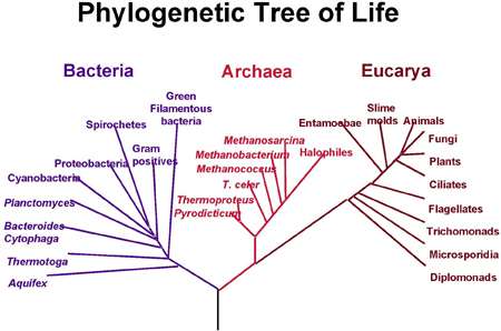
A modern phylogenetic tree. Species are divided into bacteria, archaea, which are similar to bacteria but evolved differently, and eucarya, characterised by a complex cell structure. Image courtesy NASA.
Darwin himself sketched a few phylogenetic trees in his notebooks and a little later the German biologist and artist Ernst Haeckel created a series of beautiful trees, like the one shown above. Modern phylogenetic trees are somewhat more sober-looking, but they are based on the same principle. The internal nodes represent points in time when species split into new ones. All life springs from the single common ancestor, represented by a node called the root. The species, or phylogenetic groups, as we observe them today correspond to the end-nodes at the very top of the tree, also called the leaves.
Trees like these are not only used to represent the evolution of a group of species. They can also represent the mutations of a single gene or a virus like HIV or influenza, human migration patterns, and even the development of languages.
Mathematically speaking, a tree is a set of nodes that are connected by edges in such a way that there's no more than one path between any two nodes. If an individual node has been singled out, as is the case with the common ancestral node, then the tree is called a rooted tree.If the tree splits into two at each node, then it is called a binary tree. Trees often come with numbers associated to the edges, which are called weights. In a phylogenetic tree, these weights usually quantify the amount of genetic change, for example the number of mutations of a single gene, that has taken place in the time period spanned by the edge.
To mathematicians, then, an evolutionary tree is a rooted binary tree. Mathematical trees have been studied as part of the wider field of graph theory since 1736, when Leonhard Euler published his first paper on the subject.
Figure 1: The figure on the left is a non-directed, non-rooted tree and the central figure is a binary rooted tree. Both have two interior nodes and leaves A, B, C and D. The figure on the right is not a tree, because it contains a circuit: there are two ways of going from the top interior node to the leaf A.
Reconstructing the tree of life
The big question is how to infer the correct evolutionary tree from observed data. One obvious strategy is to examine the things you're interested in, for example different species, for similarities. In Darwin's time this would have involved looking for outward resemblances like the ones between humans and apes. These days scientists look at molecular information and gene frequency data to infer similarities. Whichever method you use, one way of dealing with your information is to try and come up with a single number that quantifies the difference between any two of the objects in question.
Figure 2: A single gene has evolved through mutations. The distance between any two leaves is the number of letters that differ: the distance from A to B is 2, the distance from A to C is 3 and the distance from B to C is also 3.
As an easy example, think of the mutations of a single gene. All the information it contains is encoded by a sequence in the bases A, C, G and T, and mutation occurs through a change in the sequence: during cell division, an A in the mother cell might accidentally be copied to a G in the daughter cell. You can define the distance between any two mutations as the number of letters that differ in the corresponding sequences or, if you want to normalise your numbers, as the number of letters that differ divided by the length of the sequence.
Mathematically speaking what you get is a distance matrix: the rows and columns of the matrix are labelled by the objects of interest, and the entry corresponding to row x and column y gives the distance d(x,y) between x and y. Your aim now is to find a tree which realises your matrix: any two leaves x and y of the tree are connected by a sequence of edges and you require the weights of these edges to add up to the distance between x and y given in the distance matrix. Figure 3 shows an example of a distance matrix and a tree that realises it.
|
 |
Constructing a distance matrix isn't an exact science of course, and there's plenty of room for error. So the first mathematical question arising from this is:
Given a distance matrix, is there a tree that realises it? If yes, how many different trees are there?
From a mathematical point of view, this seems like an obvious question to ask, so it's surprising that it wasn't answered until the mid 1960s and early 1970s when several researchers came up with an answer independently. Interestingly, one of them, Peter Buneman, stumbled upon the question when trying to reconstruct the history of ancient manuscripts that, just like genes, mutate and evolve over generations as copying errors are made.
The answer lies in a generalised version of the triangle inequality: if you have three points A, B and C in the plane, then the path taking you directly from A to B will always be shorter than, or of the same length as, the path taking you from A to B via C. For a distance matrix to have any chance of representing distances between points in the plane, every triplet of points A, B and C has to satisfy the inequality d(A,B) ≤ d(A,C) + d(C,B).
The condition ensuring that there's a tree corresponding to the distance matrix involves sets of four points. It not only guarantees the existence of a tree, but also makes sure that if there is a tree, then there is only one:
The four point condition: If for any choice of four leaves A, B, C and D, the sum d(A,B) + d(C,D) is less than or equal to the larger of the two sums d(A,C) + d(B,D) and d(B,C) + d(A,D), then there is exactly one tree realising the matrix. Conversely, if there is a tree realising the matrix, then the four point condition is satisfied.
Figure 4: The four point condition - the top left figure represents a piece of a tree connecting the four leaves A, B, C and D. The other figures represent the three sums of the distances. In this image it is clear that d(A,B) + d(C,D) = d(A,D) + d(B,C), and that these two sums are greater than d(A,C) + d(B,D).
Algorithmic trees
Once you have a matrix satisfying the four point condition, you still need to reconstruct the corresponding tree. Trial and error is not an option for a large number of leaves, you need sure-fire recipes, algorithms, that are guaranteed to find the correct tree and can easily be implemented on computers. The next mathematical question is therefore:
Given a distance matrix satisfying the four point condition, is there an algorithm that is guaranteed to find the correct tree in a reasonable amount of time?
The answer is yes, luckily, but again it was only rather recently that some mathematical rigour was applied to the question. There are in fact a range of algorithms available to scientists to complete the task. One of the most popular ones is the neighbour joining method developed in the 1980s by Naruya Saitou and Masatoshi Nei. The algorithm is simple enough, but we won't go into the details here. Wikipedia has a precise description.
Saitou and Nei proved that their algorithm always gives you the correct tree as long as your distance matrix satisfies the four point condition. It is also quite efficient: for a set of n leaves the algorithm needs to perform around n3 steps. The function f(n) = n3 is what mathematicians call a polynomial — in the language of complexity theory, the problem of reconstructing a tree from data satisfying the four point condition can be solved in polynomial time.
The four point condition will no doubt delight mathematicians, but is of less immediate importance to geneticists: when you're building a distance matrix based on experimental data, it's unlikely to satisfy the four point condition exactly. There is hope, however, since in that case the algorithm will still come up with a tree that reflects your matrix reasonably well, and there are ways of quantifying just how good the resulting tree is.
Computational trees
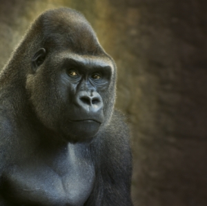
Not our closest relative. Only recently has it been confirmed that humans are evolutionarily closer to chimps than to gorillas.
The neighbour joining algorithm has the advantage of being computationally cheap, but the distance matrix approach comes with its own disadvantages. It reduces everything you know about your species or genes to a simple array of numbers, so important information may be lost. It also assumes that species that appear similar in terms of your data are also evolutionarily close. But it's easy to be fooled: a dolphin, after all, looks much like a fish, and genetic information can mislead too. The exact relationship between humans, gorillas and chimps has only recently been sorted out, after scientists disentangled conflicting evidence coming from different genes.
If you don't insist on mathematical minimalism and are happy to use some brute computational force, you can use statistical and probabilistic methods for reconstructing trees from your data. Most of these require an underlying model of evolution which estimates the probabilities that certain evolutionary changes, like mutations, occur. Equipped with such a model you can sift through a huge number of possible binary rooted trees and find the one that — in some sense — is most likely to be correct.
These methods use a lot of computing power, but they are by no means inferior to the distance matrix approach and are commonly used by scientists. A huge amount of research effort is currently going into perfecting them and assessing their effectiveness. We won't, however, go into these methods here and instead return to our elegant theory of trees.
Understanding evolutionary trees
Figuring out who evolved from what and when is in itself a rewarding thing to do, but there is a lot more you can do with an evolutionary tree once you've reconstructed it. Think, for example, of the following scenario: to augment sources of water supply to Sydney, the authorities in Australia have considered damming up some rivers in the Sydney water supply catchment region. Each river runs through a valley and each valley is home to a certain subspecies of crayfish. Damming a river upstream of the valley will have a great impact on the corresponding subspecies. The authorities know that they are able to preserve three valleys and therefore three subspecies. From an ecological viewpoint centered on the crayfish, which rivers should they choose to dam? This problem is in fact a simplified version of one encountered by the scientists Daniel P. Faith and Andrew M. Baker, published in Evolutionary Bioinformatics.
There is of course no clear-cut answer to this uncomfortable question, but one possible approach is to try and preserve as much diversity as possible: save those three subspecies that required the maximal amount of evolutionary change to appear.
How can you measure this diversity? On a phylogenetic tree, the weight of an edge represents the amount of change that occurred between the points in time represented by the two nodes connected by the edge. It encodes the diversity relating to the two nodes. In 1992, Daniel Faith suggested a way of defining the phylogenetic diversity of a set of leaves: simply find the smallest set of edges that connect all the leaves in your set, as well as the root, and add up their weights.
Figure 6: The diversity of the set A, B and C is 11.
In the example on the right, the phylogenetic diversity of the leaves A, B and C is 2+3+1+4+1=11. The crayfish question now amounts to finding the set of three subspecies that has the greatest phylogenetic diversity.
All this can easily be translated into mathematical language. If you take a set S of leaves on a tree and join them up using a minimal amount of edges from your tree, you get what is called the spanning tree of S. The weight of the spanning tree is the sum of the weights of all its edges — this corresponds to the phylogenetic diversity.
The question now becomes:
Given a tree and a whole number k (in our example k=3), is there an algorithm that is guaranteed to find the set of k leaves whose spanning tree has maximal weight?
It's another simple mathematical question, so it's again surprising that it wasn't answered until 2006, when Mike Steel and, independently, Fabio Pardi and Nick Goldman, came up with a positive answer and a rigorous proof. They showed that the greedy algorithm, so-called because it grabs the greatest numbers at each step, will always spit out the required set of leaves. Here is how it's done:
Start by picking the two leaves that are the greatest distance apart, according to edge weights. In the example below, these are the leaves B and D, because the sum of the weights of the edges connecting B and D is largest. The two leaves and the edges between them form their own little subtree, indicated in red.
Figure 7: The greedy algorithm. First join leaves B and D because they are the 'furthest away' from each other. Next join up leave A , because it will add the most weight to the subtree.
Next, look at all the other leaves in turn and add up the weights of the edges that connect a given leaf to the subtree formed by B and D. Choose the leaf for which this sum is greatest, in this case A, and connect it to the subtree, thus creating a new subtree. Repeat this process until you have a set of k leaves.
It's a straight-forward and natural approach and biologists doubtlessly knew about this greedy algorithm long before mathematicians proved its effectiveness. Coming up with a rigorous proof may seem like a purely academic exercise in this case. Something surprising happens, though, if you make the problem just a little more complex.
Suppose that each of the valleys in the crayfish example above contains more than one subspecies. Which areas should you choose to preserve now?
The difference between this and the initial problem is that you now operate with constraints: you're not looking for any old set of subspecies that maximise diversity, but for a set that corresponds exactly to a number of valleys. The set of subspecies has been carved up into groups, each corresponding to one of the valleys.
In mathematical language the problem becomes:
Suppose you have a tree whose leaves have been divided up into a number of groups. Given a whole number k, is there a polynomial time algorithm that can pick out the collection of k groups, so that the spanning tree of the leaves contained in these groups has maximal weight?
How much work did evolution put into you?
In this case, the answer is no! There is no known algorithm that can solve the problem in polynomial time. This leads to an interesting aspect of complexity theory. It's incredibly hard to prove that any given problem that appears to be unsolvable in polynomial time really is unsolvable in polynomial time — that would require you to know all possible algorithms. But mathematicians have found something quite remarkable: many complex problems for which there is no known polynomial time algorithm can be reformulated in terms of each other. If you find a polynomial time algorithm that solves one of them, you can use it to solve all of them. These problems are known as NP complete. Whether or not this illusive algorithm exists is one of the biggest open questions in mathematics. It's one of the Clay Mathematics Institute's Millennium problems and will earn the person who solves it a million dollars.
In 2006 Vincent Moulton, Charles Semple and Mike Steel proved that our constrained crayfish problem is at least as hard as the problem in the NP complete class. No hope, then, to come up with a neat shortcut solution. But not all is lost: there is a greedy algorithm that comes up with approximate results and mathematicians are able to quantify just how close they come to the optimal answer.
Lots more to do
Phylogenetics pushes the boundaries of known mathematics and more problems are sure to follow. Scientists are starting to think that Darwin's binary rooted tree may not be the best picture to have in mind. Certain species can hybridise and some bacteria can transfer genes directly from individual to individual. It may therefore be better to use more general graph theoretical objects, networks, rather than trees. Even if you do accept that evolution progresses in a largely tree-like fashion this is a useful approach. Sequencing the genome of whole organisms will soon become a matter of hours, rather than months. There will be huge amounts of genetic data and each data set can give you a different tree. Merging all possible trees into a network is a way of coping with this uncertainty, so mathematicians are currently hard at work creating the necessary network theory.
And it's not just graph theory either. Everything in phylogenetics hinges on assumptions and models and interpretation of data. Only mathematics can quantify the uncertainties involved and make sure that biologists' conclusions are statistically robust. All in all it looks as if maths and biology are finally converging. As the population scientist Joel E Cohen put it, "Mathematics is biology's next microscope, only better."
About this article
This article arose from a workshop on phylogenetics which took place at the Isaac Newton Institute for Mathematical Sciences in 2007. Many of the lectures are available on the Isaac Newton Institute website, including this webcast of a lecture given by Huson, Moulton and Steel.

Daniel Huson is Professor for Algorithms in Bioinformatics at the University of Tübingen in Germany. He is the author of a number of computer programs used in evolutionary analysis, including SplitsTree4 for computing phylogenetic trees and networks, Dendroscope for drawing large trees and MEGAN for performing taxonomical analyses of metagenomic data. All are freely available from www-ab.informatik.uni-tuebingen.de/software.

Vincent Moulton is Professor of Computational Biology and Director of the Computational Biology Laboratory at University of East Anglia. Moulton works on developing mathematical and computational techniques for phylogenetics, currently funded in part by the UK Engineering and Physical Sciences Research Council.

Mike Steel is Director of the Biomathematics Research Centre at University of Canterbury, New Zealand, and a principal investigator of the Allan Wilson Centre for Molecular Ecology and Evolution. He is co-author of the book Phylogenetics, which presents the mathematical foundation of phylogenetics.
Marianne Freiberger is Co-Editor of Plus.
Comments
mazzu
James Burr is the leading industry watcher based out of Melbourne and also mentoring businesses like www.youpack.com.au
Chris G
"Certain species can hybridise" (last para but one). The trees in this article can easily be seen in reverse as hybridisation diagrams. In Figure 2, two genes A) TTATGA and B) TTCGGA come together to reduce their differences by replacing A's third letter with B's third letter, and in return B's fourth letter is replaced by A's, to create the hybrid TTCTGA, call it H. The distance between A and B is 2, but between each of them and H is only 1.
What happens then? In the figure this H looks like it goes on to hybridise with yet another gene. But let's imagine instead that it produces three copies. Two of them are exact copies of the original A and B, and the third is an exact copy of itself, the hybrid H. This last, H's identical daughter, in turn produces only two daughters this time, but the daughters of A and B in turn produce only one each.
So far the numerical sequence representing population increase at each stage goes 2 1 3 4. with respective A:H:B ratios of 1:0:1, 0:1:0, 1:1:1, 1:2:1. Continuing to the next stage, A and B produce two copies each. One of the H's produces two but the other H only one, bringing the total to 7, with a ratio of 2:3:2. Try continuing the tree yourself.
The rule we've settled down to seems to be if your node produced two or more last generation, it gets to produce one less in this. But if it produced only one last time, then it produces two this time. The restrained rather than greedy algorithm. And maybe hybrids are a way of reducing phylogenetic distance.