
What is the Mandelbrot set?
The Mandelbrot set is generated by iteration, which means to repeat a process over and over again. In mathematics this process is most often the application of a mathematical function. For the Mandelbrot set, the functions involved are some of the simplest imaginable: they all are what is called quadratic polynomials and have the form f(x) = x2 + c, where c is a constant number. As we go along, we will specify exactly what value c takes.
To iterate x2 + c, we begin with a seed for the iteration. This is a number which we write as x0. Applying the function x2 + c to x0 yields the new number
Now, we iterate using the result of the previous computation as the input for the next. That is
and so forth. The list of numbers x0, x1, x2,... generated by this iteration has a name: it is called the orbit of x0 under iteration of x2 + c.
The theory of iterated functions is motivated by questions from real life. Modelling the growth of a population of animals is an example. The size of the population after one breeding cycle depends on how many animals there are at present, so mathematical models of population growth typically consist of a function f in a variable x, where x represents the present population size, and f(x) gives the expected population size after one breeding cycle. To work out the size of the population after any number of breeding cycles you need to iterate the function. Incidentally, the functions used in a standard model of population growth are quadratic polynomials very similar to the ones we will consider here, and this is what first motivated their study.
This leads to one of the principal questions in this area of mathematics: what is the fate of typical orbits? Do they converge or diverge? Do they cycle or behave erratically? The Mandelbrot set is a geometric version of the answer to this question.
Some examples
Let's begin with a few examples. Suppose we start with the constant c = 1. Then, if we choose the seed 0, the orbit is
and we see that points in this orbit get bigger and bigger — the orbit tends to infinity.
As another example, choose c = 0. Now the orbit of the seed 0 is quite different: it remains fixed for all iterations.
If we now choose c = -1, something else happens. For the seed 0, the orbit is
Here we see that the orbit bounces back and forth between 0 and -1. This is a cycle of period 2.
To understand the fate of orbits, it is most often easiest to proceed geometrically: a time series plot of the orbit often gives more information about its fate. In the plots below, we have displayed the time series for x2 + c where c = -1.1, -1.3, -1.38, and 1.9. In each case we have computed the orbit of 0 and marked the points in it by dots which are connected by straight line segments. Note that the fate of the orbit changes with c. For c = -1.1, we see that the orbit approaches a 2-cycle. For c = -1.3, the orbit tends to a 4-cycle. For c = -1.38, we see an 8-cycle. And when c = -1.9, there is no apparent pattern for the orbit; mathematicians use the word chaos for this phenomenon.
Figure 1: the orbit of 0 for iteration of x2 - 1.1 . The orbit approaches a 2-cycle.
Figure 2: the orbit of 0 for iteration of x2 - 1.3. The orbit approaches a 4-cycle.
Figure 3: the orbit of 0 for iteration of x2 - 1.38. The orbit approaches an 8-cycle.
Figure 4: the orbit of 0 for iteration of x2 - 1.9. There is no apparent pattern, we see chaos.
To see additional time series plots for other values of c, select a c value from the options below:
- c = -0.65 (Tends to a fixed point)
- c = -1.6 (Chaotic behaviour)
- c = -1.75 (Tends to period 3)
- c = -1.8 (Chaotic behaviour close to 3-cycle, sometimes called intermittency)
- c = -1.85 (Chaotic behaviour)
- c = 0.2 (Tends to a fixed point).
Before proceeding, let us make a seemingly obvious and uninspiring observation. Under iteration of x2 + c, either the points in the orbit of 0 get larger and larger so that the orbit tends to infinity, or they do not. When the orbit does not go to infinity, it may behave in a variety of ways. It may be fixed or cyclic or behave chaotically, but the fundamental observation is that there is a dichotomy: sometimes the orbit goes to infinity, other times, it does not. The Mandelbrot set is a picture of precisely this dichotomy in the case where 0 is used as the seed. Thus the Mandelbrot set is a record of the fate of the orbit of 0 under iteration of x2 + c: the numbers c are represented graphically and coloured a certain colour depending on the fate of the orbit of 0.
Complex numbers
How, then, is the Mandelbrot set a picture in the plane, rather than on the number line on which all the c-values we have considered lie? The answer is, instead of considering only real values of c, we also allow c to be a complex number. If you are not familiar with complex numbers, then read this brief introduction.
Let's look at some examples of the iteration of x2 + c when c is a complex number: if c=i, then the orbit of 0 under x2 + i is given by
and we see that this orbit eventually cycles with period 2. If we change c to 2i, then the orbit behaves very differently
and we see that this orbit tends to infinity in the complex plane (the numbers comprising the orbit recede further and further from the point 0, which has co-ordinates (0,0)). Again we make the fundamental observation that either the orbit of 0 under x2 + c tends to infinity, or it does not.
The Mandelbrot set
The Mandelbrot set puts some geometry into the fundamental observation above. Here is its precise definition:
The Mandelbrot set consists of all of those (complex) c-values for which the corresponding orbit of 0 under x2 + c does not escape to infinity.
The black region is the Mandelbrot set. It is symmetric with respect to the x-axis in the plane, and its intersection with the x-axis occupies the interval from -2 to 1/4. The point 0 lies within the main cardioid, and the point -1 lies within the bulb attached to the left of the main cardioid.
From our previous calculations, we see that c = 0, -1, -1.1, -1.3, -1.38, and i all lie in the Mandelbrot set, whereas c = 1 and c = 2i do not. The Mandelbrot set is named after the mathematician Benoît Mandelbrot who was one of the first to study it in 1980. The pictures below give you an idea of how incredibly intricate the Mandelbrot set is.
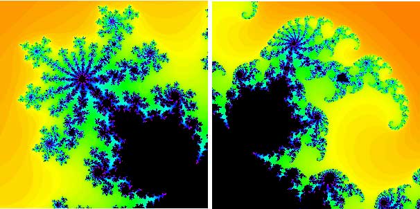
Parts of the Mandelbrot set in close-up. The two 'bulbs' shown here are directly attached to the main cardioid.
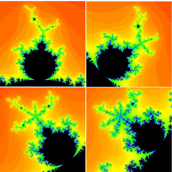
Various bulbs of the Mandelbrot set.
At this point, a natural question is: why would anyone care about the fate of the orbit of 0 under x2 + c? Why not the orbit of i? Or 2 + 3i? Or any other seed, for that matter? It turns out that there is a very good reason for inquiring about the fate of the orbit of 0; amazingly, the orbit of 0 somehow tells us a tremendous amount about the fate of all other orbits under x2 + c. To find out more about this, read the longer version of this article, Unveiling the Mandelbrot set.
About this article
This article is a shortened version of Unveiling the Mandelbrot set. You can find out more about complex numbers and things you can do with them in this introductory package and in our teacher package.

Robert Devaney is currently Professor of Mathematics at Boston University. His main area of research is dynamical systems, primarily complex analytic dynamics, but also including more general ideas about chaotic dynamical systems. He is the author of over one hundred research and pedagogical papers in the field of dynamical systems. He is also the (co)-author or editor of thirteen books in this area of mathematics, including a series of four books collectively called A Tool Kit of Dynamics Activities, all aimed at high school students and teachers. He has also been the "Chaos Consultant" for several theaters' presentations of Tom Stoppard's play Arcadia.
Professor Devaney has delivered over 1,300 invited lectures on dynamical systems and related topics in all 50 states in the US and in over 30 countries on six continents worldwide. He only needs Antartica to complete his goal of speaking on all continents — so if you teach at South Pole State and run some kind of seminar, give him a call!
Professor Devaney's website contains a number of interesting applets, articles and interactive papers on dynamical systems. Have a look.
Comments
José María Carrero
Thank you! Very nice article
Hannah
Thank you so much!! This is a fantastic explanation and really helped me understand.
Rico
I've been reading a lot of articles about the mandlebrot set because I wanted to make a simple program to draw it, and this may be the most clear explanation I've seen yet. Nicely done.
Don Oktrova
After reading the wikipedia version of this and not understanding a single thing I thought i might never be able to comprehend it... Then i read this article and everything makes sense.
Arpan Dey
When I look at the Mandelbrot set, I can't help but think that I am looking at the face of God...
Roshini P
Great explanation! Got a brief idea of what and how it works
Random math geek kid
This is so awesome! The part I don't get is how an orbital set of numbers place anything on a grid, like how does 1 2 5 26 677 458330 show a specific point? You would at least n ed an x & y right?
Random Math geek guy
Since this is an iterative function, you are not looking at a value y that is a result of a function of x. But like they said in the article, it is more representative of time-series data where we are only looking at the progression of x. However each value of x at an iteration i is not a function of i, but is based on the value of the x that came before it (x(x-1). So even though they did not label the "x-axis", it is really just a sequential progression of calculating the next value of x. So really, the "y-axis" is really the value of x calculated, and the "x-axis" is just the next iteration of calculating x.
Omer Atwood
look at the progression of x, while calculating it’s value at each iteration of I.
Okay, either way, the same pattern forms.
The problem is it’s a two dimensional representation.
If we were to calculate the pattern as a wave going out in all directions, then what appears to be infinite, is only the surface of a connected fractal. It’s Not flat. The surface of cone is finite, whoever the continuation of it, as well as the beginning of it, is made of this fractal shape.
Anonymous
can anyone suggest a good book to properly study and understand fractals?
Marianne
We found this textbook very useful https://onlinelibrary.wiley.com/doi/book/10.1002/0470013850
Mark R Simpson
This is, surely, one of the clearest texts for non-mathematically trained people to understand the beauty and power of the Mandelbrot Set. Ty