How close is close?

This is an experimental venture by the LMS, in collaboration with Plus magazine, hoping to provide a wide range of readers with some idea of exciting recent developments in mathematics, at a level that is accessible to all members as well as undergraduates of mathematics. These articles are not yet publicly accessible and we would be grateful for your opinion on the level of the articles, whether some material is too basic or too complex for a general mathematical audience. The plan is to eventually publish these articles on the LMS website. Please give your feedback via the Council circulation email address.

The notion of distance is an intuitive one, hard-wired into our brains. Without it we would not be able to move through the world; to hunt, gather, or perform any meaningful task using the opposable thumbs nature has provided us with. This is reflected in mathematics: besides counting, geometry, the study of spatial extent, is the earliest mathematical pursuit humanity has engaged in.

Mikhail Gromov came up with a brilliant way of defining distance between abstract spaces.

The distance between points in space is one thing, but we would also like to quantify the resemblance of shapes. We think of similar things as close — the faces of siblings may closely resemble each other, but can we say how far apart they are? Pinning down this type of distance exactly is tricky because there can be many aspects to compare. In the case of faces, do we want to measure the similarity of the nose, the eyes, some kind of average of the two, or neither? When it comes to measuring similarity, choices have to be made.

A step towards defining a metric to measure similarity is to place your objects into an ambient space. Facial recognition technology represents photos of faces as points in $N$ dimensional Euclidean space, where $N$ is the number of pixels in the photo and each pixel is represented by a numerical value indicating its colour. With pictures represented by points in an ambient space, it is then possible to analyse distances between them.

It is a common situation in mathematics to need to pursue abstraction — to rid our objects of an ambient context and make them stand on their own. When Bernhard Riemann developed the notion of manifolds back in the 19th century, his aim was to consider mathematical spaces intrinsically, independently of what other spaces they might be embedded in. How do we now measure the similarity of two such spaces without re-inserting them into an ambient space?

In 1981 the Russian-French mathematician Mikhail Gromov came up with a way of defining distance between abstract spaces that has been brilliantly successful in a number of very different contexts. The metric he defined, known as the Gromov-Hausdorff distance, ties together areas as diverse as Einstein's general theorem of relativity and abstract group theory and topology, and it plays an important role in Perelman's proof of the Poincaré conjecture. It was one of the many achievements that earned Gromov the 2009 Abel Prize. But before we explore his ingenious idea let's recap some basic mathematical notions of space and distance.

Metrics, spaces and metric spaces

A metric space is a set $M$ together with a function $d: M \times M \rightarrow \mathbb {R}$ which defines the distance between two elements of $M$ . The function $d$ must be symmetric, satisfy the triangle inequality, and assign a distance of zero to a pair of points if and only if the points are equal.

In the taxicab metric the blue, red and yellow paths between the two points all have the same length. The green path indicates Euclidean distance.

Euclidean space $\mathbb {R}^ n$ , with the familiar notion of distance, is of course a metric space, but other intuitive ways of defining distance give rise to metric spaces too. When in Manhattan you might want to make use of taxicab geometry, in which the distance between two points is the sum of the absolute values of the differences of their Cartesian coordinates. When travelling by rail, the British Rail Metric might be more appropriate: it defines the distance between two distinct points as the sum of their distances from London. If the points are the same, the distance is of course 0. You can verify yourself that the set of squares on a chessboard, equipped with the metric that defines the distance between two squares as the minimum number of moves a knight needs to make to get from one to the other, is also a metric space.

Once you know what it means to be close to a point in a metric space, you might want to get closer and closer, hence stumbling across the familiar notion of convergence of a sequence of points to a limit. For a general metric space there is no reason why an infinite collection of points should converge to anything at all. In Euclidean space $\mathbb {R}^ n$ , for example, one can easily find all manner of point sequences that do not accumulate anywhere: an easy example is the set of points with integer coordinates. But all the examples that first spring to mind, at least where $\mathbb {R}^ n$ is concerned, involve unbounded sequences of points, leading to the intuition that boundedness and convergence are closely related. After all, a bounded set of points cannot stray far, it must accumulate somewhere. This intuition can indeed be made precise. The Bolzano-Weierstrass theorem tells us that every bounded infinite subset $S$ of $\mathbb {R}^ n$ has an accumulation point: a point that has points in $S$ arbitrarily close to it. In other words, every bounded infinite sequence of points in $S$ contains a convergent subsequence. If $S$ is also closed, then it contains the limit of such a subsequence.

This leads us to the concept of compactness. A metric space $M$ is compact if every sequence of points within it has a convergent subsequence. As we have just seen, closed bounded subsets of $\mathbb {R}^ n$ are compact, and the converse is also true: a subset $S$ of $\mathbb {R}^ n$ is compact if and only if it is closed and bounded.

There is also a notion of compactness for a general topological space that does not involve a notion of distance. A topological space is compact if every cover of the space by open sets has a finite sub-cover. For metric spaces the two definitions of compactness are equivalent (see here for a proof).

Big and small

You can define all sorts of metrics on a topological space and it often makes sense to look for one which has some attractive geometric property such as minimising curvature in some sense. The need to minimise or maximise quantities comes up in many contexts. The best known example of such an extremal problem is provided by legend. When the soon-to-be Queen Dido arrived on the shores of North Africa having fled Tyre and her murderous brother, she asked the local ruler to give her as much land as could be enclosed by a single ox hide. She then proceeded to cut the hide into thin strips, tied them together at their ends and arranged the long strip that resulted in an arc of a circle meeting the coast at right angles. The ancient city of Carthage was founded on the terrain thus enclosed and was ruled happily by Dido until another calamity (love) befell her. If legend is to be believed then Dido had solved the isoperimetric problem: arrange a curve of a given length so that it encloses a maximal area.

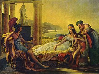
Queen Dido and her lover Aeneas.

Over 2,500 years after Dido supposedly performed her clever trick mathematicians realised that extremal problems can carry a deep physical meaning. The French mathematician Pierre Louis Maupertuis (1698-1759) was one of the first to pronounce that "nature is thrifty": physical processes (such as a body moving from A to B) that could in theory take a range of different paths will always take the one that minimises something called action, a quantity that measures the effort involved.This principle of least action has explanatory as well as predictive power: Leonhard Euler showed that it implies Newton's laws of motion. In the same spirit, and as we shall see later, Albert Einstein sought a variational principle to develop his own theory of gravity, which superseded Newton's.

In maximising or minimising a quantity you must bear in mind that the maximum or minimum may not exist. (Think of finding an ellipse of unit area whose minor axis is minimal.) What you need is a criterion ensuring that a sequence of objects for which the desired quantity gets closer and closer to its maximum or minimum does itself tend to some allowable limit. In variational problems you are often seeking to maximise or minimise an aspect of a family of functions — for example the area under their graphs — defined on a metric space. To do this, a notion of convergence of functions is crucial: if a sequence of functions converges to a limiting function, then one can hope that the aspect under consideration has a limiting value too.

There is an obvious notion of pointwise convergence: a sequence $\{ f_ n\}$ of functions defined on a common domain and with a common target converges to a function $f$ pointwise if for all $x$ in the domain the values $f(x_ n)$ converge to $f(x)$ . This is not a very useful concept, as a pointwise convergent sequence of continuous functions may converge to almost anything — something wildly discontinuous. A stronger notion is uniform convergence, which requires that the speed of convergence does not get too slow as $x$ varies over the domain. If a family of functions has the property that any bounded infinite subfamily contains a subsequence which converges uniformly on compact subsets of the domain, then it is called normal. The subsequences must then converge to continuous functions. The point of a normal family is that though it is an infinite-dimensional space of functions it has the characteristic Bolzano-Weierstrass property of finite-dimensional Euclidean spaces.

We would like to know what property of a family of continuous functions will ensure that it is normal. This crucial property is equicontinuity.

Looking at a point $x$ in the domain and a function $f$ in the family, we know that for any $\epsilon$ , sufficiently small balls around $x$ map entirely into the $\epsilon$ -ball around $f(x)$ . Just how small that ball centred on $x$ needs to be is a measure of how much the function $f$ expands things around the point $x$ — how big its derivative is, if it is differentiable. If there is a uniform bound for the expansion – if for a given $\epsilon$ there’s a limit to how small the ball around $x$ needs to be — simultaneously for all functions $f$ and all points $x$ — then the family is said to be equicontinuous.

The Arzelà-Ascoli theorem states that a family of continuous functions between two compact metric spaces is normal if and only if it is equicontinuous. This is particularly useful in complex analysis, where the derivative of a holomorphic function is bounded in terms of the function itself by Cauchy’s integral formula. For holomorphic functions between domains in the complex plane the Arzelà-Ascoli theorm gives us Montel’s theorem, which states the family is normal if it is uniformly bounded: that is, there is a number $N>0$ such that $|f(z)| < N$ for all $f$ in the family and all $z$ in the domain.

Bernhard Riemann (1826 - 1866) came up with the notion of manifolds and also with a (flawed) proof of the Riemann mapping theorem.

An interesting application of these results is the Riemann mapping theorem, first stated and proved by Bernhard Riemann in his PhD thesis in 1851. It states that any simply-connected domain $U$ of the complex plane can be mapped holomorphically and bijectively to the unit disc $\mathbb D = \{ z \in \mathbb C : |z| < 1 \}$ (although Riemann himself also imposed the condition that the boundary of $U$ be piecewise smooth). It’s a powerful result, but unfortunately Riemann’s initial proof, based on a minimisation argument, was flawed. It had relied on Dirichlet’s principle: the idea that a continuous function defined on the boundary of a domain can be extended to a harmonic function $f$ in its interior, which was justified by the fact that a harmonic function $f$ is one which minimises its energy (i.e. the integral of $||{\rm grad} f ||^2$ ) among all differentiable functions $f$ with the given boundary values. Riemann and his contemporaries believed that the principle held, but Karl Weierstrass later pointed out the unsoundness of the argument.

The first correct proof of the theorem was given in 1912 by Constantin Carathéodory, but the real breakthrough came ten years later when Leopold Fejér and Frigyes Riesz realised that the result could be proved in a single page using an extremal argument involving derivatives. Their proof uses Montel’s theorem to show that the (non-empty) family of holomorphic and injective maps $f$ from $U$ into $\mathbb D$ which take a given point $a \in U$ to 0 is normal, and so contains a function $f$ which maximises $|f^\prime (a)|$ . If $f$ isn’t surjective, then a construction invented by Carathéodory and Paul Koebe produced another element of the family whose derivative at $a$ had a larger modulus, thus deriving a contradiction.

Distance and similarity

Make a nice drawing for Hausdorff distance.

Let us now return to one of our basic questions: how do we decide if two subsets of a metric space are "close"? Should we define the distance between two subsets $X$ and $Y$ of a metric space $M$ to be the largest distance between a point of $X$ and a point of $Y$ ? This would not make much sense: if $X = Y$ then clearly we would want their distance to be zero, yet the largest distance between two points in $X$ is not zero (unless $X$ consists of a single point). Conversely, you could consider the smallest distance between a point of $X$ and a point of $Y$ . But then you would get a distance of zero if $X$ and $Y$ intersect, even if they are not equal, so this doesn’t work either.

In 1914 the German mathematician Felix Hausdorff came up with a mixture of the two approaches which does work. Firstly, given $\epsilon > 0$ , take all the points that lie within $\epsilon$ of some point in $X$ . This gives you the $\epsilon$ -neighbourhood $X_\epsilon$ of $X$ :

$X_\epsilon = \bigcup _{x \in X} \{ z \in M : d(z,x) \leq \epsilon \} .$

The $\epsilon$ -neighbourhood $Y_\epsilon$ of $Y$ is defined in the same way. The Hausdorff distance between compact subspaces $X$ and $Y$ is defined to be the smallest $\epsilon$ such that $X$ is contained in $Y_\epsilon$ and $Y$ is contained in $X_\epsilon$ :

$d_{H}(X,Y) = \inf _{\epsilon > 0}\{ X \subseteq Y_\epsilon \ \ \mbox{and} \ \ Y \subseteq X_\epsilon \} .$

We need to assume the spaces are compact, otherwise no such $\epsilon$ need exist. It’s pretty easy to see that if $X=Y$ then $d_{H}(X,Y) = 0$ , and because a compact subset is necessarily closed the converse is true also. In fact the set of all compact subsets of $M$ equipped with $d_ H$ is a metric space in its own right. (Note that the Hausdorff distance between subsets of a metric space $M$ depends on the underlying metric $d$ of $M$ , so we should really write it as $d_ H^ d$ rather than just $d_ H$ .) Equipped with a notion of distance, we can define convergence of a sequence $\{ K_ n\}$ of compact subsets of a metric space in the usual way.

Matching shapes

A small Hausdorff distance between two sets means that the sets are not only close to each other in the ambient space, but also that they are in some sense similar metric spaces. (Only "in some sense", because the subset $S_ n$ of the unit interval $I = [0,1]$ formed by the $n+1$ points $\{ 0,1/n,2/n,3/n, \ldots , 1\}$ has distance $1/2n$ from $I$ , and converges to $I$ as $n \to \infty$ .) In any case, the converse is far from true. Two sets $X$ and $Y$ could be identical in shape, for example they could be two circles with the same radius, but they could still be far away from each other in terms of Hausdorff distance, for example if the circles are centred on different points. To decide how similar the two shapes are irrespective of where they are located in space we need another notion of distance — one that doesn’t need any ambient space at all.

To derive it, start with some intuition. Suppose you have a perfectly round circle $X$ drawn on a transparency and a slightly squashed circle $Y$ drawn on a second transparency. To see just how much $Y$ is deformed compared to $X$ you can glue the transparency with $X$ on it to your table top and then slide the $Y$ transparency around until you get the best fit.

Felix Hausdorff (1868-1942).

Now imagine that as you are sliding the $Y$ transparency I shout "stop" and you stop. You’ve now got two sets $X$ and $Y$ both sitting anchored in 3D Euclidean space. Even if they overlap, they don’t strictly speaking intersect as they are drawn on two different transparencies. You can now work out the Hausdorff distance between the two. This gives you a whole set of possible Hausdorff distances, one for every location on the table of the $Y$ transparency. The best fit of $X$ and $Y$ occurs when this Hausdorff distance is minimised; when the $Y$ transparency sits on the $X$ transparency so that the two shapes overlap as much as possible.

Here we are still dealing with the ambient Euclidean space, of course, but we can generalise the idea using the notion of the disjoint union of sets. So let’s suppose our two sets $X$ and $Y$ are each a compact metric space in its own right with metrics $d_ X$ and $d_ Y$ respectively. We don’t have an ambient space, so let us just consider the disjoint union $Z$ of $X$ and $Y.$

You can define all sorts of metrics on $Z$ , but we are only interested in the set $\mathcal{D}$ of metrics $d_ Z$ on $Z$ that reduce to $d_ X$ and $d_ Y$ when restricted to the individual components $X$ and $Y$ . Each of $X$ and $Y$ is isomorphically and canonically embedded in $Z$ in the obvious way. Now given $d_ Z \in \mathcal{D}$ you can work out the Hausdorff distance

$d_ H^{d_ Z}(X,Y)$

of $X$ and $Y$ in their disjoint union. The Gromov-Hausdorff distance between $X$ and $Y$ is defined to be the infimum of the Hausdorff distances

$d_ H^{d_ Z}(X,Y)$

over all metrics $d_ Z$ in $\mathcal{D}$ :

$d_{GH}(X,Y) = \inf _{d_ Z \in \mathcal{D}}d_ H^{d_ Z}(X,Y).$

It turns out that $d_{GH}(X,Y)=0$ if and only if $X$ and $Y$ are isometric (i.e. if there is a distance-preserving bijection between them). Now we can consider the set of all compact metric spaces and identify two metric spaces if they are isometric, to get the set of all isometry classes of compact metric spaces. One can prove that $d_{GH}$ turns this into a metric space. With this notion of distance we can define what we mean by a sequence of compact metric spaces converging to another compact metric space.

Remembering how useful the Arzelà-Ascoli theorem was for spaces of functions, we ask: is there a sufficient condition that ensures that a sequence $\{ X_ i\}$ of compact metric spaces has a convergent subsequence? It is clear that the set of diameters of the spaces must be bounded. An example of a sequence with unbounded diameters that does not converge to any compact metric space is a nested sequence of concentric discs in the plane whose radii tend to infinity — this sequence is "trying" to converge to the whole plane, which isn’t compact, and so isn’t allowed.

But boundedness is not enough. Think, for example, of the nested sequence formed by the closed unit balls $B^ n$ in $\mathbb R^ n$ , as $n \to \infty$ . We need stronger constraints. Returning to our transparency example, it is clear that any shape drawn on a transparency can be approximated by covering it with as few discs of a certain radius $\epsilon$ as possible. As $\epsilon$ gets smaller, the approximation becomes more accurate. Now suppose you have a family of metric spaces, and suppose that for a given $\epsilon$ there is some number $N_{\epsilon }$ such that each of the spaces can be covered by at most $N_\epsilon$ $\epsilon$ -discs. This condition rules out the sequence of balls $B^ n$ of increasing dimension, because the $2n$ ends of the coordinate axes in $B^ n$ are at distance greater than 1 from each other, so $B^ n$ needs at least $2n$ balls of radius 1/2 to cover it. (The same argument shows that the condition also rules out families of spaces of unbounded negative curvature. For the unit disc in a surface of constant negative curvature – $k^2$ has circumference $2\pi (\sinh {k})/k$ , which tends rapidly to infinity with k. Negative curvature will play an important role in the next two articles.)

Does the existence of such a universal upper bound $N_\epsilon$ for all $\epsilon > 0$ give us enough constraint to guarantee that a subsequence of our spaces converges in the Gromov-Hausdorff metric? It is a startling fact that it does indeed. This is the basic version of Gromov’s famous compactness theorem.

As we mentioned in the introduction the Gromov-Hausdorff metric has proved incredibly useful. In the next article we will examine one of its applications as a vital tool in the proof of a major conjecture, not in geometry, but in abstract group theory.

Add new comment