
Not just a matter of time: Measuring complexity
As computers are constantly becoming faster and better, many computational problems that were previously out of reach have now become accessible. But is this trend going to continue forever, or are there problems computers will never, ever be able to solve? Let's start our consideration of this question by looking at how computer scientists measure and classify the complexity of computational algorithms.
Classifying complexity

How complex is complex?
Suppose you are responsible for retrieving files from a large filing system. If the files are all indexed and labelled with tabs, the task of retrieving any specific file is quite easy — given the required index, simply select the file with that index on its tab. Retrieving file 7, say, is no more difficult than retrieving file 77: a quick visual scan reveals the location of the file and one physical move delivers it into your hands. The total number of files doesn't make much difference. The process can be carried out in what is called constant time: the time it takes to complete it does not vary with the number of files there are in total. In computers, arrays and hash-tables are commonly used data structures that support this kind of constant time access.
Now suppose that over time the tabs have all fallen off the files. They are still indexed and in order, but you can no longer immediately spot the file you want. This introduces the requirement to search, and a particularly efficient way to do so is a binary search. This involves finding the middle file and seeing whether the file you need comes before or after. For example, when looking for file 77, pull out the middle file and see if its index is smaller or larger than 77, and then keep looking to the left or right of the middle file as appropriate.
Big O notation
Write $S(n)$ for the number of steps required to solve a problem of size $n$ using a particular algorithm (e.g. searching for a file within a total number of $n$ files using binary search). Let $f(n)$ be a function of $n$ (e.g. $f(n) = \log{(n)}$). Then we say that $S$ has complexity, or order, $O(f(n))$ if there is a positive number $M$ so that for all $n$ sufficiently large $$S(n) \leq Mf(n).$$With this single step you have effectively halved the size of the problem, and all you need to do is repeat the process on each appropriate subset of files until the required file is found. Since the search space is halved each step, dealing with twice as many files only requires one additional step.
Writing $n$ for the total number of files, it turns out that as $n$ grows, the number of steps it takes to solve the problem (that is, the number of steps it takes to find your file) grows in proportion to $log(n),$ the logarithm to base $2$ of $n$ (see the box below to find out why). We therefore say that a binary search is logarithmic, or, alternatively, that it has computational complexity $O(\log{(n)}).$ This is the so-called big O notation: the expression in the brackets after the O describes the type of growth you see in the number of steps needed to solve the problem as the problem size grows (see the box on the left for a formal definition).
A logarithmic time process is more computationally demanding that a constant time process, but still very efficient.
Logarithmic growth
Suppose the total number $n$ of files to be searched is equal to a power of $2$, so $n = 2^k$ for some natural number $k$. At each step you halve the number of files to be searched. If you are unlucky you need to keep on halving until you have reached $1$ and can halve no longer. What's the maximum amount of times you can halve $2^k$ before you hit 1? It's $k$ — and $k$ is of course the logarithm to base $2$ of $n$. The number of files might not be an exact power of $2$ of course, but the big O notation only indicates that the number of steps needed to complete the algorithm grows in proportion to $log (n)$. It doesn't have to grow exactly like $log(2).$But what if over time the loss of the tabs has allowed the files to become disordered? If you now pull out file 50 you have no idea whether file 77 comes before or after it. The binary search algorithm therefore can't be used. The best option in this situation is a linear search, where you just go through the files one by one to find the one you need. The complexity of this search increases in line with the number of files, and so it is an $O(n)$ process.
Clearly it was better when the files were sorted, so eventually you decide to put them all back in order. One way to manage this is by selecting each file in turn, starting from the front, and comparing it with all earlier ones, moving it forward until you find the place it belongs in the order. In this way the sorted order is rebuilt from the front, file by file. This simple sorting algorithm requires $O(n^2)$ steps (you can try and work out for yourself why this is true). And it brings us into the realm of polynomial time complexity. An expression of the form $n^k,$ where $k$ is a natural number ($k=2$ in our example) is called a polynomial in $n$. A polynomial time algorithm is one of order $O(n^k)$ for some $k.$This last example is the infamous and inefficient Bubblesort, and the number of comparisons required gets very big very fast. Fortunately many more efficient sorting techniques exist, such as Quicksort, and Mergesort, each with complexity $O(n \log{(n)}).$ To see the difference this reduction in complexity makes, consider that for $100$ files, Bubblesort requires $100^2=10000$ comparisons on average, whereas Quicksort only needs around $100\log{(100)} \approx 665$ and so is about 15 times faster. For $1000$ files, Quicksort is more than $100$ times faster (thus reducing each minute of runtime to sub-second), and the advantage becomes even greater as $n$ increases.
Travelling further along this path of increasing complexity we come to exponential time algorithms with complexity $O(k^n)$ for some constant $k.$ An example is a brute-force search for password strings of length $n$ from $k$ possible characters: for each character of the password you have $k$ choices, giving a total of $$\underbrace{k\times k\times ... \times k}_n = k^n,$$ possible passwords. Slower still are factorial complexity algorithms $O(n!).$ Here the expression $n!$ stands for $$n! = n \times (n-1) \times (n-2) \times ... \times 2 \times 1,$$ and grows very fast with $n.$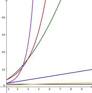
The complexity hierarchy: the black line illustrates zero growth (constant time), the yellow line logarithmic growth, the blue line linear growth, the green line polynomial growth, the red line exponential growth and the purple line factorial growth.
The famous travelling salesman problem provides an example of such an algorithm: the task is to find the shortest road circuit that visits each of $n$ given cities exactly once. A naïve solution involves generating and checking all possible paths through every town and it weighs in at $O(n!).$
These examples illustrate the complexity hierarchy for problems of size $n$ where $k$ is a constant greater than 1, $O(1) O(\log{(n)}) O(n) O(n^k) O(k^n) O(n!),$ where $O(1)$ stands for constant time. Constant time problems are the easiest to solve, followed by $O(\log{(n)})$ problems, and so on, all the way up to $O(n!).$In complexity theory, any algorithm with complexity described by a polynomial in $n$ or less is considered tractable, and anything with greater complexity intractable. Finding polynomial time algorithms for problems where the only known algorithms require non-polynomial time is therefore of major interest. In fact, there is a whole class of important problems where no polynomial time algorithm is known. Finding one, or, conversely, proving that none exists, is the most important open problem in computer science (the P vs NP problem, see this article to find out more).
Some huge examples
Some well known puzzles provide a powerful illustration of the growth rate of the exponential function. One example is asking
How thick would a regular piece of paper be if you could somehow fold it 42 times?
The answer is quite astounding – it would reach the Moon! (Indeed, fewer than 100 folds would be necessary to reach the limits of the visible Universe.) Another is the ancient wheat and chessboard problem that asks

How many grains are on the last square?
How many grains of wheat would be needed to enable you to place 1 grain on the first square of a chessboard, 2 grains on the second, 4 grains on the third, and so on, doubling each time until all squares have been used?
The repeated doubling means this is an exponential process, and the 64th square will contain $2^{63} = 9 223 372 036 854 775 808$ grains of wheat.
Factorial growth is even faster. Consider the number of arrangements of a pack of cards. The first card chosen in any arrangement is one of 52. The next choice is one of the remaining 51, then one of the remaining 50, and so on until every card has been chosen. The total number of arrangements possible is therefore $$52! = 52\times51\times50\times ... \times1, $$ or $$80658175170943878571660636856403766975289505440883277824000000000000.$$
Scott Czepiel beautifully describes the magnitude of this number on this website. One of his illustrations involves imagining that you start a timer to count down this many seconds, and begin to walk around the equator, taking just a single step every billion years. Then, each complete circuit, remove a single drop of water from the Pacific Ocean and start around the Earth again. When you have emptied the ocean, place one piece of paper flat on the ground, refill the ocean and start yet again. Repeat until the stack of paper reaches the Sun, then look at the timer to see how far it has counted down. The first three digits will not even have changed. The entire process must be repeated thousands of times before the counter reaches 0.
These examples illustrate why problems with solutions of such complexity are considered intractable. But such a consideration is rooted in practical concerns. What if we propel ourselves into an ideal future, to a time when we'll have all the computing power we need and no limits on storage? In the second part of this article, we will look at functions that grow much faster than exponentials and factorials, and see what implications such functions have for idealised computability.
About the author

Ken Wessen has PhDs in Theoretical Physics and Human Biology, and a Graduate Diploma in Secondary Mathematics Education. He has taught both at university and in high schools, but most of his working life has been in investment banking, developing algorithms for automated trading of equities and foreign exchange. In his spare time he writes free software and develops online activities for mathematics learning at The Mathenaeum.