The physics of language (continued): matrix statistics

Research in natural language processing (NLP) began in the areas of linguistics, computer science and artificial intelligence. As we saw in the previous article, the main intention was to use machine learning methods to gather these large datasets in order to attempt to automatically extract the meaning of the words in the language.

But when Sanjaye Ramgoolam, a theoretical physicist from Queen Mary, University of London, came to the wealth of data NLP had produced, he naturally brought with him his perspective from physics. He looked at the data as a kind of evidence from the experiment of analysing all the natural language texts. "Language is a complex system, so maybe some ideas from complex systems in physics could work," he says.

A physicist's perspective

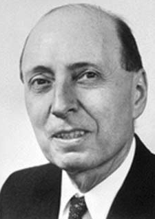
Eugene Wigner.

"Whenever you have data, you want to understand the nature of the noise in it. From a statistical point of view we have an interesting collection – maybe 100,000 adjectives – and it's nice to know where this data sits. If one word is an outlier – what kind of outlier is it?" This was a totally new approach to NLP – no one had been thinking about doing these sorts of statistics on the data sets before. But studying the statistics of collections of matrices was already an important technique in physics.

"People had studied collections of matrices in physics before. This is called random matrix theory," says Ramgoolam. One of the first applications was to understand the energy levels of complex nuclei, such as uranium and other heavy materials. "The nuclear force is very complex. It's not really possible to calculate the energy levels of uranium from first principles – we don’t know how to do that – but we can measure these experimentally."

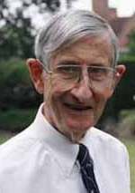
Freeman Dyson (Photo and copyright Anna N. Zytkow)

The physicists Eugene Wigner and Freeman Dyson realised that you could get interesting physics by studying the statistics of all the evidence from your experiments on nuclei. "They had the idea that we don't understand what is going on [in each individual nucleus], so let's study the statistics of the whole ensemble," said Ramgoolam. In quantum mechanics, the energy levels of anything is related to a matrix, called the Hamiltonian, that describes the system you are studying. So studying the statistics of experimental results about energy levels, means that you are studying the statistics of a corresponding collection of matrices.

"As a physicist, the reason for studying the statistics of these matrices is that maybe there's some simplicity in the whole that isn't there in each matrix. And that's why I got interested in the statistics of these matrices."

It's normal to be Gaussian

As Ramgoolam explained, when you have a nice big data set you can use statistics to get an understanding of where the data is, which values are typical and which values are outliers. An obvious first step to understanding this is calculating the average, or mean: the sum of all the observed values, divided by the number of observations.

Let's consider a simple data set consisting of the heights $x_1, x_2, \ldots , x_ n$ of $n$ people. If you make a histogram of the data, showing how many people there are of each recorded height, you'd expect to get the bell-shaped curve centred on the mean height, $\bar{x}$ .

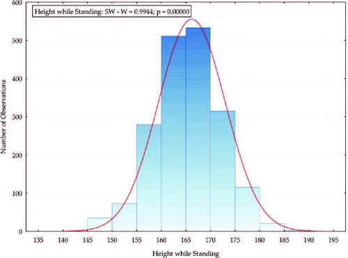A histogram, showing how many people there are of each recorded height. (Figure from Hitka et. al. 2018 – CC BY 3.0)

The mean, $\bar{x}$ , helps you locate the data. Another measure, called the variance, $v$ , helps you quantify how spread out your data is. You can think of the variance is like the average of the squared distances for each observed value from the mean:

$v = \frac{1}{n}((x_1-\bar{x})^2 + (x_2-\bar{x})^2 + \ldots + (x_ n-\bar{x})^2).$

The standard deviation, written $\sigma$ , the square root of the variance, gives a more direct sense of how spread out the observed values are around the mean. If your data is distributed in a bell curve, like the one above, it is said to have a normal or Gaussian distribution. In a Gaussian distribution we have a really good idea of where a typical value would be: over 68% of the values are within one standard deviation from the mean, over 85% within two standard deviations from the mean, and less than 0.3% are more than 3 standard deviations from the mean.

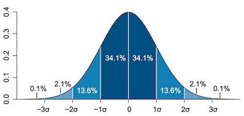
The Gaussian distribution showing the standard deviations. (Image by M. W. Towes - CC BY 2.5)

Taking the moments

All sorts of data sets we come across from real life are distributed in this way: the Gaussian distribution is one of the most ubiquitous, and most useful distributions in statistics. One of the key features of the Gaussian distribution is that it is completely described by just two numbers: the mean and the standard deviation. These numbers uniquely define the shape of the curve describing the Gaussian distribution of your observed values.

You need more numbers, called moments, to describe a more complicated curve. You can think of the first, or linear moment, $<x>$ , as a generalisation of the mean: the average of the values $x$ that you observed, only that there can be several first moments while there can only be one mean. The variance, and the associated standard deviation, are related to the average of the squares of your observations of the value $x$ . You can think of the second, or quadratic moment, $<x^2>$ , as a generalisation of the standard deviation.

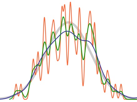
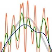
You can extend this idea and think of the third or cubic moment, $<x^3>$ , as an average of the cubes of your observations of the value $x$ . You can think of the fourth or quartic moment, $<x^4>$ , is the average of your observations of $x$ raised to the power of 4. You can continue on in this way calculating higher and higher moments from your observed values in your data. "These moments uniquely describe the curve [of the distribution of your data]," says Ramgoolam. "As you change the curve, you change the moments."

The shape of the Gaussian curve, shown in light grey, is defined by the first and second moments. As you vary these and the higher moments, you change the shape of the curves, shown in colour. (Image from M. W. Toes – CC BY-SA 4.0)

The curve of the Gaussian distribution is uniquely defined by the first and second moments, because for a Gaussian curve all the higher moments can be written in terms of the first and second moments. "Once you know it's a Gaussian distribution, and once you know the mean and standard deviation, you know all the higher moments."

We can also use this information to go in the opposite direction: if we have a dataset we can test if it fits a Gaussian distribution. You can calculate the higher moments theoretically, in terms of the first and second moments, according to a Gaussian distribution. Then you can check these theoretical predictions of the higher moments against the experimental data.

Ramgoolam had decades of experience using Gaussianity in theoretical physics to understand and predict the behaviour of a physical system. But could he do the same thing for language? Find out in the next article...

Sanjaye Ramgoolam explains how he is using techniques from physics to give new insight into language

About this article

Dr Sanjaye Ramgoolam is a theoretical physicist at Queen Mary University of London. He works on string theory and quantum field theory in diverse dimensions, with a focus on the combinatorics of quantum fields and the representation theory of groups and algebras. One of his recent research directions, sharing some of these mathematical mechanisms, is the development of an approach to the study of randomness and meaning in language.

Rachel Thomas is Editor of Plus.