Solution to Puzzle No. 8

September 1999

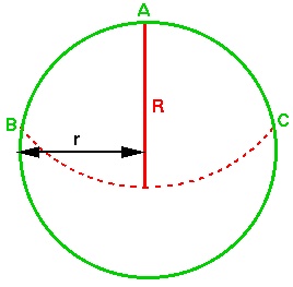
For the question see Puzzle No 8 - The Gobbling Goat in issue 8.

Let the circular field have radius $r$ .

Let the length of the rope, which is anchored at point $A$ on the circumference of the field, be $R$ .

Now, with the rope at full stretch, the goat will be able to move in an arc from point $B$ on the circumference to point $C$ .

Let $O$ be the centre of the field.

Clearly, the angle $OAB$ is equal to the angle $OAC$ . Let the magnitude of $OAB$ be $x$ radians.

Thus, the area accessible to the goat will be a circle sector with radius $R$ and angle $2x$ (yellow), plus two circle segments (pink) from a circle of radius $r$ , cut off by the chords $AB$ and $AC$ respectively.

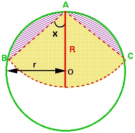
Now, the area of the circle sector is:

${1\over 2} (R^2 . 2x) = R^2x$

The area of each circle segment is:

$(1/2)r^2(\pi -2x) - (1/2)r^2\sin (\pi -2x)$

(because each is a sector of a circle minus a triangle) and so the total area accessible by the goat is:

$R^2x + r^2[\pi - 2x - \sin (2x)]$

(the yellow sector plus the two pink segments).

Currently, we have two different variables in our area equations: $r$ and $R$ . Let’s try to eliminate one.

Obviously, the length of the line segment $AO$ is $r$ , the radius of the field. Similarly, the radius of the line segment $OC$ must be $r$ .

Therefore, by similar triangles, if we drop a perpendicular from $O$ to the line segment $AC$ , the perpendicular will bisect $AC$ . Therefore the length of $AP$ (and $PC$ , of course) is $R/2$ .

We now have a right-angled triangle and enough information to calculate the relationship between $r$ and $R$ :

	$\displaystyle \cos x$	$\displaystyle =$	$\displaystyle R/(2r)$		(1)
	$\displaystyle R$	$\displaystyle =$	$\displaystyle 2r \cos x$		(2)

So the total area accessible to the goat is:

$(4r^2\cos ^2 x)x + r^2[\pi - 2x - \sin (2x)] .$

We wish for this area to be half the area of the total field; therefore we have:

$\displaystyle 4r^2 x \cos ^2 x + r^2[\pi -2x-\sin (2x)]$	$\displaystyle =$	$\displaystyle \pi r^2/2$
$\displaystyle 4x \cos ^2 x + \pi - 2x - \sin (2x)$	$\displaystyle =$	$\displaystyle \pi /2$
$\displaystyle 4x \cos ^2 x + \pi /2 - 2x - \sin (2x)$	$\displaystyle =$	$\displaystyle 0$

We can't easily solve the equation but we can use a graphical calculator or numerical method such as Newton-Raphson to find an approximate solution.

Using the Newton-Raphson method as described in the Coda, we find that

$x$ is approximately $0.953$ , and therefore $\cos x = 0.579$ .

Now, since $R = 2r \cos x$ and $r$ , the radius of the field, is 100m, we have $R = 200 \cos x$ and thus the required length of rope is approximately 116m.

Coda: Solving the equation using Newton-Raphson

The basic idea

In the goat puzzle, we were left with the following equation to solve:

$4x \cos ^2 x + \pi /2 - 2x - \sin (2x) = 0$

The Newton-Raphson method is an approximate method for finding roots of equations that are differentiable.

Let $f(x)$ be a differentiable function. Since $f(x)$ is differentiable, every point on the graph of $f(x)$ must have a gradient and a unique tangent line.

Now, the tangent at $x_0$ is an approximation to the graph of $f(x)$ near the point $(x_0,f(x_0))$ .

Therefore the zero of the tangent line (the point where the tangent line crosses the $x$ -axis) is an approximation (perhaps a very bad one, however!) of the zero of $f(x)$ (the point where $f(x)$ crosses the $x$ -axis, i.e. the root of $f(x)$ ). It’s like we’re pretending that $f(x)$ is really a straight line, like the tangent line, and therefore crosses the $x$ -axis at the same place the tangent does.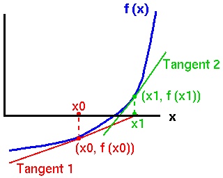

In the Newton-Raphson method, we start with a "best guess" $x_0$ as to the zero of $f(x)$ . We then calculate the first approximation, $x_1$ , as the zero of the tangent line to $f(x)$ at $x_0$ .

We then calculate the second approximation, $x_2$ , as the zero of the tangent line crossing the $x$ -axis at $x_1$ , and so forth.

The diagram above shows the initial guess $x_0$ , the first approximations $x_1$ and the relevant tangents. The second approximation $x_2$ is the coordinate where the second tangent crosses the $x$ -axis. As you can see, the approximations are getting closer to the actual zero point of $f(x)$ . If we continue iterating like this, we will get better and better estimates for the zero point of $f(x)$ .

How do we do it?

We wish to solve $4x \cos ^2 x + \pi /2 - 2x - \sin (2x) = 0$ . Obviously, plotting $f(x) = 4x \cos ^2 x + \pi /2 - 2x - \sin (2x)$ and drawing tangents is not going to be very much fun! However, we can perform Newton-Raphson numerically.

Our initial point is $x_0$ . The gradient of $f(x)$ at $x_0$ is given by $f’(x_0)$ , and the tangent line to $f(x)$ at $x_0$ is therefore given by:

$y - f(x_0) = f’(x_0) (x - x_0)$

To find $x_1$ , we must find the point where this tangent crosses the $x$ -axis, i.e. to let:

$0 - f(x_0) = f’(x_0) (x_1 - x_0)$

and therefore

$x_1 - x_0 = \frac{-f(x_0)}{f'(x_0)}$

so that

$x_1 = x_0 - \frac{f(x_0)}{f'(x_0)}$

Similarly, in the general case we obtain:

$x_{n+1} = x_ n - \frac{f(x_ n)}{f'(x_ n)}$

Now, our function is $f(x) =4x \cos ^2 x + \pi /2 - 2x - \sin (2x)$ . Via standard differential calculus, the gradient $f’(x)$ of this function is

$4 \cos ^2 x - 8x \cos x \sin x - 2 - 2 \sin (2x) \cos (2x).$

Therefore, to find the approximate root of $f(x)$ we can use the following:

$x_{n+1} = {x_ n} - \frac{4x_ n \cos ^2 x_ n + \pi /2 - 2x_ n - \sin (2x_ n)}{4\cos ^2 x_ n - 8x_ n \cos x_ n \sin x_ n - 2 - 2 \sin (2x_ n) \cos (2x_ n)}$

So, we know how to calculate $x_{n+1}$ from $x_ n$ . But how do we find our starting value, $x_0$ ? Well, in this particular case we know that the magnitude of $x$ must be between 0 and $\pi /2$ radians (go back to the second diagram and think about it if you’re not sure why!). So a good initial guess might be (for example) $\pi /4$ .

As it turns out, all sorts of values will do: here’s a table of the iterative steps of Newton-Raphson on our function $f(x)$ for a range of initial values of $x_0$ . As you can see, they all converge quite rapidly to the same twelve-significant-digit approximation.

	$x_0 = \pi /4$	$x_0 = \pi /6$	$x_0 = \pi /3$	$x_0 = \pi /2$
$x_0$	0.785398163397	0.523598775598	1.047197551200	1.570796326790
$x_1$	0.967088277214	1.254847487960	0.956164730983	0.785398163397
$x_2$	0.953058379193	0.966611488070	0.952884951928	0.967088277214
$x_3$	0.952849994306	0.953049230238	0.952848237620	0.953058379193
$x_4$	0.952847886046	0.952849901115	0.952847868401	0.952849994306
$x_5$	0.952847864870	0.952847885110	0.952847864693	0.952847886046
$x_6$	0.952847864657	0.952847864860	0.952847864655	0.952847864870
$x_7$	0.952847864655	0.952847864657	0.952847864655	0.952847864657
$x_8$	0.952847864655	0.952847864655	0.952847864655	0.952847864655
$x_9$	0.952847864655	0.952847864655	0.952847864655	0.952847864655

Add new comment

You can simplify the equation by using the cos(2x) trig identity

Comment

4 x cos^2(x) + pi/2 - 2x - sin(2x) = 0
can be simplified a little using cos(2x) = 2 cos^2(x) - 1
You get:
2 x cos(2x) + pi/2 - sin(2x) = 0
or replacing variables (y = 2x):
y cos(y) + pi/2 - sin(y) = 0