101 uses of a quadratic equation: Part II
In 101 uses of a quadratic equation: Part I in issue 29 of Plus we took a look at quadratic equations and saw how they arose naturally in various simple problems. In this second part we continue our journey. We shall soon see how the humble quadratic makes its appearance in many different and important applications.
Let us begin where we left off, with the quadratic curves known as the circle, ellipse, hyperbola and parabola. These were known and have been studied since the ancient Greeks, but apart from the circle they did not seem to have any practical application. However, in the 16th century the time came for them to change the world.
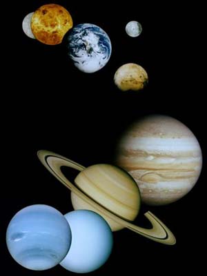
Image courtesy of NASA
With the coming of the Renaissance, deep thinkers started to look at the world in a different way. One of these was Copernicus, who made history by proposing that the Earth went round the Sun rather than the other way round. Copernicus thought that the orbit of the Earth was a circle - partly because it is very close to a circle, and also because the circle, being so symmetric, was regarded as the most perfect possible curve. Things stayed like this until Kepler, using some very careful observations of Tycho Brahe, found some discrepancies between the predictions of Copernicus' theories and the experimental data. What Kepler discovered was that the planets did not go round the Sun in circles, instead they went round in ellipses. Kepler's rules then fitted the observations perfectly. At last the conic sections that we saw in the last article came into their own, 1500 years after they were discovered. Politicians and newspaper journalists please take note! It didn't stop there: other celestial objects, such as certain comets, were found to move along hyperbolic orbits. These remarkable discoveries by Kepler helped to usher in the modern world.
Quadratic equations not only described the orbits along which the planets moved round the Sun, but also gave a way to observe them more closely. The key to further advances in astronomy was the invention of the telescope. Using a telescope Galileo was able to observe the moons of Jupiter and the phases of Venus, both of which gave support to the Copernican theories. Later on, great reflecting telescopes were used to probe the mysteries of the Universe. In recent years, giant radio telescopes have been used both to listen for aliens and to send messages which a potential alien might pick up. Galileo's telescope used lenses, the shape of which was formed by two intersecting hyperbolae. The reflecting telescope, invented by Newton (see later) has a mirror for which each cross section takes the shape of a parabola! The same parabolic shape works just as well for the bowl of a giant radio telescope, a shaving mirror and a satellite TV dish. Truly, quadratic equations lie at the heart of modern communications.
Galileo, why quadratic equations can save your life and 'that' drop goal
The fit between the ellipse, described by a quadratic equation, and nature seemed quite remarkable at the time. It was as though nature said: "Here is a curve that people know about, let's make some use of it." Understanding why this was the right curve had to wait till Galileo and then Newton. The answer is perhaps the single most important reason that quadratic equations matter so much: it is the link between quadratic equations and acceleration. It was Galileo who first spotted this link at the beginning of the 17th century.

Quadratic equations are necessary for an understanding of acceleration. Image freeimages.co.uk
Most people have heard of Galileo, a colourful Professor of Mathematics at the University of Pisa. The final part of his career centred on an epic battle with the Spanish Inquisition on the validity of the Copernican view of the solar system. However, before this he devoted much of his life to a study of how things move. Long before Galileo, the Greek scientist Aristotle had stated that the natural state of matter was for it to be at rest. Aristotle also said that heavier objects fell faster than lighter ones. Galileo challenged both of these pieces of accepted wisdom. At the heart of Galileo's work was an understanding of dynamics, which has huge relevance to such vital activities as knowing when (and how) to stop our car and also how to kick a drop goal.
At the heart of this is an understanding of the idea of acceleration and the role that quadratic equations play in it.
If an object is moving in one direction without a force acting on it, then it continues to move in that direction with a constant velocity. We can call this velocity $v$. Now, if the particle starts at the point $x=0$ and moves in this way for a time $t$, then its resulting position is given by $x = vt.$ Usually the particle has a force acting on it, such as gravity for a rugby ball or friction in the brakes of a car. Fast-forwarding to Newton we know that the effect of a constant force is to produce a constant {\em acceleration} $a$. If the starting velocity is $u$, then the velocity $v$ after a time $t$ is given by $v = u + at$. Galileo realised that you could go from this expression to working out the position of the particle. In particular, if the particle starts at the position $x=0$ then the position $s$ at the time $t$ is given by \[s = ut + \frac{1}{2} at^2. \] This is a {\em quadratic equation} linking $t$ to $s$ with many major implications for all of us. For example, suppose that we know the braking force applied to a car: then this formula allows us to work out either how far we travel in a time $t$, or conversely, solving for $t$, how long it takes to travel a given distance. \par A very important application is to find the {\em stopping distance} of a car travelling at a given velocity $u$. Suppose that a car is travelling at such a speed, and you apply the brakes, how long will it take to stop? Even journalists might be interested in this question, especially if it means avoiding an accident. In particular, if a constant {\em deceleration} $-a$ is applied to slow a car down from speed $u$ to speed 0, then solving for $t$ and substituting gives the stopping distance $s$: $$s = \frac{u^2}{2a}.$$
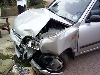
Even a journalist might care. Image freeimages.co.uk
The reason that this result is so important for all of us is that it predicts that doubling your speed quadruples, rather than doubles, your stopping distance. In this quadratic expression we see stark evidence as to why we should slow down in urban areas, as a small reduction in speed leads to a much larger reduction in stopping distance. Solving the quadratic equation correctly here could, quite literally, save your, or someone else's, life!
The simple quadratic formula relating time to distance is also the basis of the science of ballistics, which looks at the way that objects move under gravity. In this case, an object falls in the $y$ direction with a constant acceleration $g$. In contrast, it moves in the $x$ direction horizontally at a constant velocity (in the absence of air resistance). If it starts at the point $x = y = 0$ with velocity $u$ in the $x$ direction and velocity $v$ upwards, then Galileo was able to show that the position at time $t$ is given by $$x = ut \quad \mbox{and} \quad y = vt - \frac{1}{2} g t^2.$$ Put another way, we have $$y = \left( \frac{v}{u} \right) x - \left( \frac{g}{2u^2}\right) x^2,$$ yet another quadratic equation, this time relating $x$ to $y$. What was remarkable was that the resulting shape of the trajectory was, of course, a {\em parabola}.
Suppose now that you are in the final minute of a rugby match and you have to kick a perfect drop goal. To do this you must kick the ball at the correct angle and velocity so that when it travels a distance x to the goal it is at the right height y to go over the goalposts. To do this you must solve a quadratic equation. Of course in the heat of the moment you may not have time to do this, which is where practice comes in! More seriously, the parabolic equation for the particle trajectory - with modifications to allow for air resistance, the spin of the projectile and also the spin of the Earth - serves as the basis for artillery calculations...a fact not lost on the military following Galileo's discovery.
We leave Galileo with the discovery of the pendulum. Around the year 1600, Galileo was attending a church service in Pisa (he had to). Bored by the sermon, he started watching a chandelier swing to and fro - and made a remarkable discovery: the time taken for a swing of the chandelier was independent of its amplitude. This discovery led to the invention of the pendulum and various timepieces such as the Grandfather clock, but at the time Galileo could not explain it. To do so we need another quadratic equation.
Newton, quadratic equations and singing in the shower
Newton was born in the year that Galileo died and went on to totally transform the way that we understand science and the role that mathematics plays in scientific predictability. Newton was inspired by the work of both Galileo and Kepler. These scientific giants had accurately described phenomena of dynamics and celestial mechanics, but neither had formulated scientific explanations. It was left to Newton to provide the mathematical explanation of the phenomena that they observed.
Firstly, he formulated the three laws of motion, which explained Galileo's observations. Secondly, he described the fundamental law of gravitation, which was that two masses were attracted to each other by a force inversely proportional to the square of the distance between them. By using geometrical arguments he was able to prove that such a law of force implied that the planets had to move around the sun in a conic section. (Of course, it was a tremendous fluke that the inverse square law led to orbits which could be explained in terms of known curves!) Newton also worked in the field of optics, and recognised that the telescopes that Galileo had used (based on lenses) caused problems by refracting light of different colours in different ways. He overcame this by designing a telescope based on a mirror. The best shape for the mirror, to bring all points into focus, was none other than the parabola, leading to the reflecting telescopes we saw earlier.
However, Newton had further aces up his sleeve. While he used geometrical arguments to explain things to his contemporaries, he had also (in parallel with Leibnitz, but independently from him) developed calculus. This was a mathematical theory of the way that things change and it was perfect for describing objects acting according to his laws of motion. The fundamental device in the application of calculus to the real world is the differential equation, which relates the change in the conditions of an object to (for example) the forces acting on them. Differential equations are at the heart of nearly all modern applications of mathematics to natural phenomena, from understanding how heat flows through a bar to the way that animal coat patterns develop (see How the leopard got its spots, also in this issue of Plus). Their applications are almost unlimited, and they play a vital role in much of modern technology.
When Newton was alive this was all still in the future! But one problem he did consider was the motion of the pendulum which so interested Galileo. This motion can be described in terms of a differential equation, and in the case of small swings of the pendulum this equation can be solved to find the time of the swing. Solving it requires finding the solution to a quadratic equation!
If $x$ is the angle of swing of the pendulum, then Newton realised that there were numbers $a,b$ and $c$ which depend on such features as the length of the pendulum, air resistance and the strength of the gravitational force so that the differential equation describing the motion was $$a\frac{d^2 x}{dt^2} + b \frac{dx}{dt} + cx = 0.$$ Here $t$ is time, $\frac{d^2 x}{dt^2}$ is the acceleration of the pendulum and $\frac{d x}{dt}$ is its velocity.
It is possible to find approximate solutions to equations such as this by using a computer, and this is the approach generally used for the very complex differential equations encountered in modern technology. However, the mathematician Leonhard Euler devised a means of solving this particular equation that relied on the solution of a quadratic equation. Euler suggested the existence of a solution of the form $$x(t) = e^{wt},$$ where $e = 2.718281828... $ is the basis of natural logarithms. The importance of this function is that $$ \frac{d\ e^{wt}}{dt} = we^{wt}.$$ Substituting into the differential equation and dividing by $e^{wt}$ gives the following equation for $w$: $$aw^2 + bw + c = 0.$$ This is very familiar! All we need to do to solve the original differential equation is to solve this quadratic equation and substitute back for $w$. By doing this we can accurately predict the behaviour of the pendulum.
What is also fascinating is that the different types of solution of the quadratic equation lead to quite different solutions of the differential equation. If b2>4ac, then the quadratic equation has two real solutions.
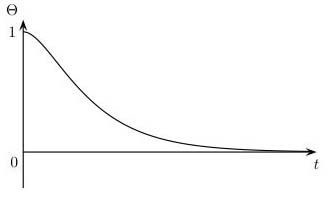
The same differential equation has a solution looking like the diagram to the right. Physically this solution corresponds to a pendulum with a lot of friction (or a pendulum moving in a liquid such as water).
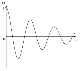
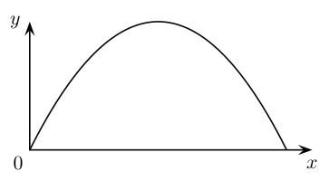
In contrast, if b2<4ac, then the same differential equation has oscillating solutions which look like the diagram to the left. These are more like the motions of the pendulum that we are familiar with.
The difference between these two types of motion is very profound and occurs because, in the second case, the solutions of the quadratic equation are complex and involve the square root of -1. We will look at these in more detail presently.

The new karaoke
The discovery that differential equations of this sort (they are called second order constant coefficient equations) can be solved by using quadratic equations has extraordinary importance. The reason is the universality of differential equations, and the fact that the solutions of the resulting quadratic equation tell us whether the solutions are likely to grow, stay the same size, or get smaller. This is very important to engineers who are trying to design safe structures and machines. In these structures, small disturbances which grow will rapidly lead to structural failure (called instability). Very similar considerations apply to electrical circuits. In practice, often it is by solving the above quadratic equation and finding whether the roots w have certain properties that a safe machine can be designed. Sometimes growing solutions can be useful, especially when linked to the phenomenon of resonance. Imagine that you vibrate the pendulum up and down at a frequency of f. Certain values of f lead to much larger responses than others. This is resonance. You encounter resonance every time that you tune a radio or sing in the shower. It is the resonant notes of the shower that sound the best (and loudest) when you sing them. In the case of the swinging pendulum, the resonant frequency is given by $$f = \sqrt{c/a}.$$
Quadratic equations take to the air
The link between quadratic equations and second order differential equations is no coincidence: it is all tied up with the link between force and acceleration described in Newton's second law. When Newton formulated this law he was thinking mainly of the motion of rigid bodies. However, it was soon realised that the same laws could be applied to the way fluids such as water and air moved. In particular, it is possible to use Newton's laws to find relationships between the speed of a fluid and its pressure. Sophisticated versions of these laws (called the Navier-Stokes and related partial differential equations) are solved on large computers to forecast the weather. However, a particular solution, valid for many types of fluid flow, was one of the key ingredients in the discovery of the basic principles of flight. The consequences of this have been immeasurable and are linked (as ever) with a quadratic equation called the Bernouilli equation.

Quadratic equations take to the air. Image DHD Photo Gallery
The Bernoulli family comprised many mathematicians who both individually and together made enormous advances in mathematics. One of them, Jacob Bernoulli, looked at the way air moved. He discovered that if you look at the steady flow of air with speed $u$ and pressure $P$, and an air particle is moving at a height $h$, then there is a constant $E$ (the {\em energy} of the air particle) so that $$\frac{u^2}{2} + P = h.$$ Significantly, if $h$ is constant then this formula predicts that if $u$ increases then $P$ decreases. This is called the Bernouilli effect. This result is a direct consequence of Newton's laws of motion and only applies to smoothly moving fluids which are not too sticky (viscous). However, this quadratic equation is accurate enough to predict the behaviour of the flow of air over the wing of an aircraft and to see why an aircraft flies.
There are a number of simple experiments which can demonstrate the Bernoulli effect. One of the simplest is to suspend two ping-pong balls on cotton thread a couple of centimetres apart. Then blow gently between them and watch what happens. Rather than being blown apart, they move together.
This shows that the pressure exerted by a fluid (the air) decreases as the speed of the fluid increases. You might expect a moving fluid to exert more pressure, but here we are talking about the lateral pressure, not the force generated by the momentum of the fluid itself. That is the force you feel when the wind blows.
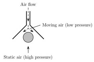
A more extreme experiment, which really works, involves another ping-pong ball. This is released from rest in an upside-down funnel with a downward air flow.
If you use a steady flow of the air and a big enough funnel, you should be able to balance the ping-pong ball. In practice a backwards vacuum cleaner, a ping-pong ball and a large kitchen funnel work very well indeed. This looks very odd as the downdraft of air seems to suck the ball up. However, it is perfectly in agreement with the physical principle!
Why a complex quadratic equation leads to the mobile phone
Let us pause and think for a moment about what happens when we square a number: that is to say, when we take $x$ and calculate $x^2$. One thing we notice is that, no matter what value we take for $x$, $x^2$ is always non-negative. As a consequence, $x^2=-1$ cannot have a solution. The way mathematicians coped with this problem was to cheat and just define a solution into existence! The letter $i$ is used to represent a solution to \[x^2=-1,\] so $i^2=-1$. So, $i$ can't be a real number and because of this it is called an {\em imaginary number}. Notice also that \[ (-i)^2 = -1 \times i \times -1 \times i = i\times i = -1. \] So $x=-i$ is also a solution to the equation $x^2=-1$.
Historically, imaginary numbers first came to light when trying to solve cubic equations, rather than quadratics. What was most perplexing was that in using these subtle and imaginary numbers it was possible to solve cubic equations. In fact, the case that needed imaginary numbers during the calculation turned out to have real solutions!
This mathematical fix needs to be justified! Otherwise we might just keep inventing new kinds of numbers every time we encounter a problem we can't solve. Eventually we would run out of letters, and in any case we would gain no understanding of how all these new kinds of numbers related to each other. The whole thing would be hopeless. The very deep mathematical result is that actually inventing new kinds of numbers turns out to be quite unnecessary. Using a combination of real and imaginary numbers, known as complex numbers, turns out to be sufficient to solve virtually all mathematical problems! The first person to really use imaginary numbers with confidence was Leonhard Euler, who lived from 1707 to 1783, and one of his other wild and daring mathematical calculations is explained in An infinite series of surprises by one of us (Chris Sangwin) in issue 19 of Plus.
The imaginary number $i$ occurs in one of the most beautiful formulas in mathematics, which relates $\pi$, $e$ (the base of the natural logarithms) and $i$. This is \[e^{i\pi}=-1.\] This is a special case of a more general result, which links the exponential function $e^x$ with $\sin(x)$ and $\cos(x)$ via complex numbers. Euler discovered that \[ e^{it}=\cos(t)+i\sin(t). \] Both $\cos(t)$ and $\sin(t)$ are oscillating terms, which is to say they repeat periodically. This formula provides an insight into how the differential equation which modelled the damped pendulum, which has a solution of the form $e^{wt}$, can have oscillating solutions. If $w$ is imaginary, or complex, Euler's formula allows the exponential term to be rewritten as a combination of $\sin(t)$ and $\cos(t)$. \par Another very significant application of the imaginary number $i$ to the physical world comes from quantum theory. This theory deals with phenomena at a microscopic level where quantities (such as electrons or photons of energy) can behave both like particles and oscillating waves. As we have seen, oscillating behaviour can be described using $i$. The fundamental equation of quantum theory which is used to calculate the "wave number" of a quantity (the probability of it being in a particular location) is Schr\"odinger's equation. This is a (partial) differential equation involving $i$, which can be written as \[ i \frac{\partial u}{\partial t} + \nabla^2u +v(x)u=0.\] This equation has very many practical applications. By using it to predict the motion of the electrons and holes in semi-conductors it is possible to design integrated circuits with huge numbers of components which can perform amazingly complex tasks. Such circuits are at the heart of much modern technology, including computers, cars, DVD players and mobile phones. Indeed, a mobile phone works by converting your speech into high frequency radio waves and the behaviour of these waves can then be calculated using further formulae involving $i$. So we can say with justification that without the simple quadratic equation $x^2=-1$ the mobile phone would never have been invented.
A touch of quadratic chaos
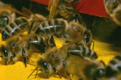
Imagine you are a biologist or ecologist who is interested in the way the population of a particular species of insect changes from year to year. Some insects have only one generation per year, and a simple model assumes that the population in the next year will depend only on the population in the current year. So, if xn is the population in year n, then xn+1 will be some function of xn.
One very simple model assumes that a proportion, axn, say, breed successfully and that bxn2 die from overcrowding. To simplify the equations we may re-scale the coordinates to obtain the following quadratic equation:
xn+1 = rxn(1-xn)
for some fixed number r >0 and initial population x1. Strictly speaking, we have defined a whole family of quadratics, labelled by the constant r. Each member of this family is known as a logistic map.
It is well worth performing some numerical experiments to investigate the behaviour of these insect populations. You can try these yourself using a spreadsheet such as Excel. To do this place the initial population into cell A1, which should be between 0 and 1. Then, type the formula
= 4*A1*(1 - A1)
into the cell A2. This has the effect of making A2 equal to the population in year 2, given a value of r=4. Now, copy the contents of the cell A2 into A3, A4 and so on. The great thing about Excel, and other spreadsheet packages, is that it automatically changes the reference to A1 in the formula to the cell above. Then Excel will automatically calculate the insect population for a number of years. You can change the initial population in cell A1. You can also change the value of r, which in the case of the example above was set to 4. If this is done, you will have to copy the new formula into all the cells again. The adventurous can also plot the values of the insect population on a graph.
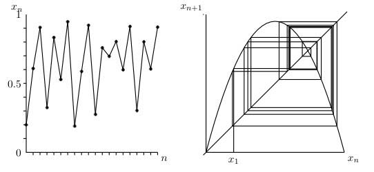
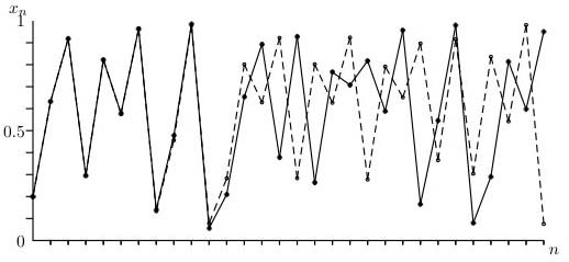
The figure above shows the logistic map with x1=0.2 and r=3.7. Notice the very complex-looking and unpredictable behaviour from the system. To the left is a graphical plot. The image to the right is known as cobwebbing, since it looks a bit like a spider's web. This is a graphical procedure to help you visualize the behaviour of insect populations.
To draw a cobweb plot, the first thing to do is choose the value of r and then plot the quadratic on the cobweb diagram. Then the initial population, x1 on the x-axis and also the line y=x. The value of x2 is rx1(1-x1) by definition, which is just the value of x1 on the graph. So draw a vertical line from x1 until it hits the graph. Next draw a horizontal line from x2 to the line y=x. Now we have the position of x2 on the x-axis and can repeat the process. To find x3, we can just draw another vertical line to the graph, and then a horizontal line back to the line y=x. This graphical procedure can be repeated, without becoming blinded by lists of numbers. You can get an excellent sense of what is going on with a cobweb diagram.
The interactive applet below will allow you to experiment with different values of r by pulling the maximum of the quadratic up and down. The maximum turns out to be r/4 in the logistic map, and so the applet allows you to use r between 0 and 4. You can also change the initial population by pulling the horizontal bar with the mouse.
Java Applet by Dr. A. D. Burbanks
These quadratic logistic maps demonstrate chaos, which is a modern and exciting area of applied mathematics. Chaos is used to describe a system which behaves in an apparently random way, even when the system itself is not random. What is most surprising is that:
Very simple systems behave in very complex ways.For example, below we show what happens when you take two initial populations that are very close together. In particular we start the system with x1=0.2 and then x1=0.2001, which are very close indeed. After only a few generations the populations are doing completely different things! This kind of behaviour would be a disaster if you wanted to forecast the populations, but had to estimate the initial populations.
Actually, chaos says a lot more. Indeed, if you make any error at all in estimating the initial insect populations then very soon your prediction will be hopelessly wrong. You should try some experiments yourself using a computer and the logistic map with r=4 to get a feeling for how this works. As you will discover, not all values of r will produce chaos. So instead of trying to forecast the insect population, which may be impossible, scientists and mathematicians try to understand when a particular system is chaotic. Knowing this allows us to know when a prediction is accurate and when it is hopeless. For more examples of chaos, see Finding order in chaos by Chris Budd, from issue 26 of Plus.
Conclusion
We have shown that the quadratic equation has many applications and has played a fundamental role in human history. Here are a few more applications in which the quadratic equation is indispensable. As a challenge, can you make this list up to 101?
That drop goal, grandfather clocks, rabbits, areas, singing, tax, architecture, sundials, stopping, electronics, micro-chips, fridges, sunflowers, acceleration, paper, planets, ballistics, shooting, jumping, asteroids, quantum theory, chaos, windows, tennis, badminton, flight, radio, pendulum, weather, falling, shower, differential equations, telescope, golf.
I'm not scared of you any more!
Afterword
This article was inspired in part by a remarkable debate in the British House of Commons on the subject of quadratic equations. The record of this debate can be found in Hansard, United Kingdom House of Commons, 26 June 2003, Columns 1259-1269, 2003.
About the authors
Chris Budd is Professor of Applied Mathematics in the Department of Mathematical Sciences at the University of Bath, and the Chair of Mathematics at the Royal Institution in London.
Chris Sangwin is a member of staff in the School of Mathematics and Statistics at the University of Birmingham. He is a Research Fellow in the Learning and Teaching Support Network centre for Mathematics, Statistics, and Operational Research.
They have recently written the popular mathematics book Mathematics Galore!, published by Oxford University Press.
Comments
Anonymous
What a great page! I will probably come back to this for when I teach high school math :) Once I pass that dang CSET of course
Anonymous
I'm only in 8th grade and this is an awesome website and your students will learn a lot from this page. It may be a super long page but it has a ton of information..
Anonymous
This page is awesome
Anonymous
That's all I can say after reading this article. I am just trying to understand the concept of quadratic equations and am blown away by your explanation. It made it a little easier for me.
thanks,
pady
Anonymous
Great article, many thanks. I'm assuming we're modelling electrons in semi-conductors, not elections.
luke@mathsbank.co.uk
Marianne
Yes indeed! Thanks for spotting the typo, we'll correct it.
Anonymous
I have shared this with my son who is doing his IB , and is awed with the new learning ...It will help him to enjoy Maths and link to real world and not just study for exam .
Anonymous
this really useful for my young brothers. Some days before He asked me how to implement this equation in daily life. this will help him understand the use of this equation in daily life.
Anonymous
Very nicely written and explained.
Anonymous
Big gaps for me here. Need some practical examples each step of the way. Anywhere I can find them?
T. Simmons
Anonymous
I am sorry but the application of bernouli's theorem top the ping pong ball example and also to aircraft flight is completely erroneous. Air moving in an air strean has exactly the same pressure throughout. (Check many corrections on the internet for this effect).
The reason the balls move together is that the Coanda effect causes the air stream to follow the curve of the ball which gives the air a component of accelleration away from the centre - because air has mass Newtons laws requires a force to be responsible for this component of acceleration and it is this force which draws the balls together. The same explanation applies to the upper wing surface of an aircraft
Anonymous
Because Galileo was Italian, the Galileo Affair had nothing to do with the Spanish Inquisition, which, not surprisingly, took place in Spain. Furthermore, Galileo's trouble with the Church was not a result of his science but rather a result of him making theological pronunciations based on his scientific observations and theories.
Anonymous
If you read the actual sources you will find that Gallileo not making "theological pronunciations" but was simply elaborating on his scientific observations. The church at the time was denying the validity of the science that Galileo was espousing. To say his position was theological is like saying that assertions of climate change are theological.
Anonymous
superb explanation.keep it up..!!!!!!!!!!!!! :-) :-)
Anonymous
Very nice article! Was looking for some material to inspire high school student to solve quadratics, and this is super helpful!
One comment though --- I don't quite agree with the portayal of imaginary numbers. There is no "cheating" involved in defining a number system where i = sqrt(-1). The only reason x^2 > 0 for real x is because we have _defined_ multiplication that way. We ourselves make these rules about number systems, and we're free to make new ones; hence, the imaginary numbers are not more strange or "illegal" than anything else in mathematics. At some point in time, people were also uncomfortable with the idea of subtracting a larger number from a smaller one, because it was felt that negative numbers "don't exist". And the same can be said for irrational numbers.
Personally, I think the terminology "real" and "imaginary" numbers is unfortunate. The truth is of course that *all* numbers are imaginary; they exist only in our imagination!
Anonymous
Well all that we use are the complex numbers. Here, on an argant plane every point depicts a relation which is the subset of real x imaginary. Complex set is the supreme set and the greatest discovery in mathematical world.
Anonymous
Thanks, you have explained more than my math teacher has in the last 3 months
Anonymous
Was looking for practical examples of the Quadratic formula and this has been very informative.
David Scoins
Would you please add a page explaining and demonstrating the uses of what I call related equations. A-level Maths has long included, towards the harder end of the course, exploring equations with related roots. E.g if an equation has roots p and q, what equation has roots 1/p and 1/q. I can see advantage in learning to manipulate algebra reliably so as to do this, but wondered what it was historically that prompted such work. I wondered whether the approach was indirect - I can't solve , but I can solve , so the original answer ought to look like ...? I expect part of the reply to come from differential equations, but is the non-maths bit that intrigues me - the maths, I can do that.