Skill or chance?

In the previous article A League Table Lottery we began exploring the treacherous territory of league tables by looking at the National Lottery. The underlying process was random in that case, yet a league table based on its outcomes still showed up potentially misleading patterns. This time we look at tables based on non-random processes, representing some of the most important and the most emotive league tables we come across: performance tables for schools and hospitals, or the football league, for example. Yet, as football fans will know, especially those backing losing teams, chance has a hand in these areas too, as success or failure can depend on a range of random factors. How informative are league tables in these cases, and can the inherent uncertainty be quantified? We'll investigate using the example of the Premier League.

The Premier League is the main English football league, with 20 teams each playing a home and away game against each of the others, making 38 matches for each team in a season, and 380 matches altogether. Teams are awarded 3 points for a win, 1 point for a draw and 0 points for losing. The league position is decided on total points. If two teams have an equal number of points, the ranking will be decided by goal difference: the number of goals scored minus the number of goals conceived. At the end of the season the top team carries off the trophy while the bottom three teams are relegated to a lower league.

We can use the history of the Premier League table over the 2006-2007 season to see how the spread of points develops.

The table below shows the points accumulated by the teams in the 2006-2007 season.

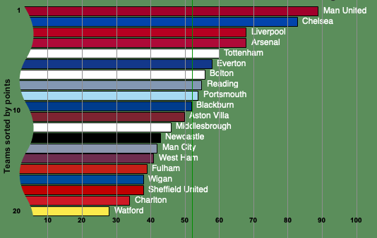
Manchester United won that particular season while Watford, Charlton Athletic and Sheffield United were relegated. To see to what extent the final table reflects the teams' quality, we'll compare it to a table produced by chance alone.

What distribution of points would you get by chance alone?

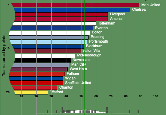
The spread of points at a particular time in the season can be visualised by a histogram. On the horizontal axis mark all the total scores a team could possibly have achieved so far. These range from 0 to the maximal number resulting from a team winning all its matches up to this point. Against each of these possible scores, plot the number of teams that have achieved that particular score.

Now assume that the league is decided purely by chance: all teams are of equal standard and the matches are decided at random. It's possible to work out a theoretical distribution which reflects the spread of points you'd expect assuming randomness (a little more on this follows below). The figure below again shows the 2006-2007 league table, but this time we have included the corresponding histogram (in grey) and the theoretical distribution (in white) at the bottm. It's clear that the actual and theoretical distributions differ quite strongly — we can conclude that there are genuine differences between the teams. To find out to what extent these difference are reflected in the table, we have to use some basic probability theory and statistics.

For each, the actual league and the chance league, we'll look at two quantities: the mean, describing the average number of points per team, and the variance, describing the spread of points around this average. The two variances are the numbers we will compare, as they will tell us to what extent the observed spread is a result of chance. \\ \\ For the actual results of the 2006-2007 season the sample mean $\bar{x}$ and the variance $s^2$ are computed from our observations. Writing $x_i$ for the total number of points of team $i$ at the end of the season, we calculate the mean by adding all the $x_i$ and then dividing by the total number of teams, which is 20. This gives $\bar{x} = 52.1$. \\ The variance is given by $$s^2 = 1/n \sum_{i=1}^n (x_i - \bar{x})^2,$$ where $n$ is the total number of teams (so $n = 20$) and $\sum_{i=1}^n (x_i - \bar{x})^2$ stands for the sum of $(x_i - \bar{x})^2$ over all $i$. In our case $s^2 = 238.7$. \\ For the chance league the mean and variance are initially theoretical quantities that depend on the underlying probabilities. To compute them it helps to split the matches into home wins, away wins and draws. Suppose that the result of each match is decided at random with the probability $p_H$ of a home win, probability $p_D$ of a draw and probability $p_A$ of an away win, and $p_H+p_D+p_A=1$. Write $X_H$ for the number of points a team wins in a home match. $X_H$ is a random variable. Its mean is $$m_H = E(X_H) = 3p_H+p_D.$$ The variance of $X_H$ is given by: $$v_H = V(X_H) = E(X_H^2) - m_H^2 = 9p_H + p_D - m_H^2.$$ Similarly, writing $X_A$ for the number of points a team wins in an away match, the mean and variance are: $$m_A = E(X_A) = 3p_A+p_D,$$ $$v_A = V(X_A) = E(X_A^2) - m_A^2 = 9p_A + p_D - m_A^2.$$ If in a season a team plays $N/2$ home matches and $N/2$ away matches, then the total points $T$ at the end of the season is the sum of all the points in the individual matches, and so has mean and variance $$m_T=E(T)=\frac{N}{2}(m_H+m_A)=\frac{N}{2}(3(p_H+p_A)+2p_D)=\frac{N}{2}(3-p_D),$$ $$v_T=V(T)=\frac{N}{2}(v_H+v_A)=\frac{N}{2}(9(p_H+p_A)+2p_D-m^2_H-m^2_A)=\frac{N}{2}(9-7p_D-m^2_H-m^2_A).$$

To get some actual numbers for these values, we have a look at past records. These indicate that overall 48% of matches are home wins, 26% draws, and 26% are away wins — this will be called the 48/26/26 law. We can use these values to estimate the probabilities, so $p_H =0.48$, $p_D =0.26$ and $p_A=0.26$. The total number $N$ of matches played by each team is 38. This gives $m_T = 52.06$ and $v_T = 61$. \\ \\ The sample mean and the theoretical mean are very close, but this is only part of the story. It's the spread of points that signifies a difference between the actual league and the chance league, and this is measured by the variance in each case. To compare the variances we take the quotient 61/238.7. This is roughly equal to 0.25, so we conclude that 25\% of the variance in the Premier League points is due to chance. The standard deviation of the observed points, which is the square root of the variance, is roughly equal to 15, while that of the random points is around 8. This means that the observed points have about twice the range of the random points.

How sure can we be about the true quality of each team?

The end-of-season point totals describe how well each team has performed, but since chance did have a considerable part to play, they do not quite reflect the true underlying quality of each team. There is a way, however, to gain more information from our league table.

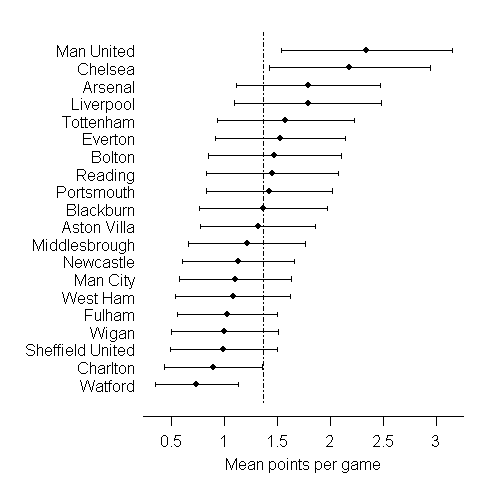
For each individual team, the average number of points per match only gives a glimpse of the team's quality: we'd get a much better idea if the team had played, say, 38,000 or 380,000 matches, rather than just 38. Let's therefore imagine that the season continues indefinitely and that after an infinite number of matches we can work out the average, or mean number $m$ of points per match scored by an individual team. We can regard this theoretical quantity as a true measure of the team's quality. The actual point average per match for the team, as observed in the 2006-2007 season, is an estimate of this true measure. It is worked out by adding the team's points at the end of the season and dividing by the total number of matches the team played, which is 38. Probability theory gives a way of assessing our confidence in one particular estimate. Without going into too much detail, the main idea here is to regard the difference between the theoretical quantity $m$ and the observed point average of the team as a random variable (for which we'll write $D$): each time we take a sample, in other words observe the team play a run of matches, we'll get a different value for the point average over these matches, and so $D$ can take on a range of possible values. In most cases, the distribution of $D$ will be unknown, so we don't know how likely it is that $D$ takes on a particular value. However, amazingly, there are powerful results from probability theory stating that, if our sample is large enough, then the distribution of $D$ can be approximated by a distribution we do know.\\ Using these ideas it is possible to estimate the probability of $D$ lying within a certain range, say between -2 and 2. It's also possible to stipulate the probability first and then find the corresponding range. For example, it's possible to find a value $a$ so that the probability of $D$ lying within the interval from $-a$ to $a$ is 0.95. This is equivalent to saying that the probability of the observed point average lying within $a$ of the theoretical value $m$ is 0.95. When we observe a point average, then the values of $m$ within a distance $a$ give a confidence interval with a confidence level of, in our example, 95\%.\\ \\ The table below shows the 95\% confidence intervals for each team. In each case we are 95\% confident that the theoretical value $m$, the true measure of the team's quality, lies within the interval shown. From this it is clear that only Manchester United and Chelsea can be reasonably claimed to be better than average, while we can be confident that Charlton and Watford are below average.

How sure can we be about the appropriate rank of each team?

Once we take the final average number of points per game as an estimate of an unknown quality measure, it becomes reasonable to view the observed rank of the team in the league table as an estimate of the true underlying rank of the team. Computer simulations from distributions based on the intervals shown above allow us to make predictions of thousands of "possible worlds" in each of which we can imagine the league fixtures going on and on until we are really certain of the "true ranking" of each team. The variability in these possible true rankings can be summarised as an interval around the current observed rank. The table below shows the teams on the vertical axis, plotted against their rank on the horizontal axis. For each team, we are 95% confident that the true rank lies in the interval shown.

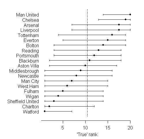
There is huge uncertainty as to the true ranks of the teams: this is typical of many applications of league tables. Manchester United and Chelsea again come up as the only teams we can be reasonably sure are in the top half of the table, while only Watford can be confidently placed in the bottom half.

We can also consider the probability that the season's winner, Manchester United, really was the best team: this works out to be 53%, compared to 31% for Chelsea. This could be interpreted as the probability that Chelsea would actually end up top of the league table were the season to continue indefinitely.

Were the teams that were relegated really the three worst teams? The probability of being one of the bottom three teams works out as 77% for Watford, 47% for Charlton Athletic, and 30% for Sheffield United. Wigan and Fulham narrowly escaped relegation, and in fact each has a 28% probability of truly being one of the bottom three teams.

The lesson is simple: if we are going to use league tables as a true measure of quality, then we have to serve them up with a lot more statistical information than is usually given.

About this article

Many more examples about the way that chance comes into sport can found in Beating the Odds: The Hidden Mathematics of Sport by Plus authors Rob Eastaway and John Haigh.

David Spiegelhalter is Winton Professor of the Public Understanding of Risk at the University of Cambridge. Mike, David and the rest of their team have created the Understanding uncertainty website to inform the public about the mathematics of chance, risk, luck, uncertainty and probability.