Modelling nature with fractals
Computer games and cinema special effects owe much of their realism to the study of fractals. Martin Turner takes you on a journey from the motion of a microscopic particle to the creation of imaginary moonscapes.
Brownian motion in Nature
It was a Scottish botanist Robert Brown who noticed the near random movement of a small particle when it is immersed in a liquid or gas. The liquid or gas is composed of continually moving molecules that hit the small particle from different directions. This movement is now named after him and called Brownian motion. A physicist Jean Perrin tried to measure the velocity which is the derivative of the particle's position with respect to time, but found that the velocity of the particle
"varies in the wildest way in magnitude and direction, and does not tend to a limit as the time taken for an observation decreases"and also said that
"nature contains suggestions of non-differentiable as well as differentiable processes".
The following pictures show a computer generated particle being observed at different time intervals. As the time intervals are reduced the calculated length of the path actually increases.
Length=6392, Step=32
The figure above shows the path of a computer generated particle. At regular time intervals the position of the particle is observed and plotted. The three figures below then show the same path but with the frequency of these observations doubling each time.
Length=8747, Step=16
Length=12091, Step=8
Length=17453, Step=4
This study of Brownian motion shows us that some processes in nature are best modelled by non-differentiable functions. These functions will have a length that is infinite.
The term fractal, introduced in the mid 1970's by Benoit Mandelbrot, is now commonly used to describe this family of non-differentiable functions that are infinite in length. As you look closer into the curve the apparent length becomes longer and longer. In the extreme this would create an infinitely long line. In reality we reach the tiny level of molecules that are pushing the particle. For those who want to find out more about differentiation and fractals take a look at "The origins of fractals" elsewhere in this Issue.
Von Koch - from Curves to Islands
One of the most famous deterministic fractals was described by Niels von Koch and is called the Von Koch Island. Consider starting with a single straight line that we will call the initiator.
The initiator
We now define a generator, or production rule, that states
"Take the initiator, scale it down by a factor r=1/3, make N=4 copies and replace the initiator by these scaled down copies, oriented as shown".
The generator

The generator is repeated...
and repeated...
and repeated...
etc...
After an infinite number of repetitions this curve will be everywhere non-differentiable and will also have infinite length. To create the Von Koch Island (also called the Von Koch Snowflake) we join three lines together to form a triangle and repeat the above process on all three sides.
Level 1
Level 2

Level 3
Surprisingly it is not too difficult to calculate the area enclosed by each level of the Island. We may define the area of the original triangle to be
At each level the small triangles added to the Island are one ninth the size of the last triangles added. At level 1 we add three of these triangles, so
After this the number of small triangles added at each level is four times the number added at the last level. See if you can work out why from the diagrams.
Hence at level 2,
and at level 3,
Repeating these steps, we see that at level n
Then as n approaches infinity we see that the area converges
So although the Island has a fractal boundary, and therefore one of infinite length, the area enclosed is finite and very well defined.
Landscapes - Mandelbrot Surfaces
The above curve is deterministic in that it always looks the same no matter how often it is created. We now add some randomness to the process and use it to create a synthetic mountain landscape.
Start with a grid of four points defining the corners. We now specify four random values that define the heights at these points, and scale the heights by a scaling factor d.
Next we divide this square up into four squares. This will define four new points around the edge of our original square, and also a point in the centre of it. The heights at these five new points are calculated as follows:
- For a given 'edge-point' we first calculate the average of the heights of its two neighbouring corners, and then add on a random value. This random value is normally distributed and scaled by a factor d1 related to the original d by

- For the point in the centre we calculate the average of all four original corners, and then add on a random value, scaled as above.
We can now carry out exactly the same procedure on each of the four smaller squares, continuing for as long as we like, but where we make the scaling factor at each stage smaller and smaller; by doing this we ensure that as we look closer into the landscape, the 'bumps' in the surface will become smaller, just as for a real landscape. The scaling factor at stage n is dn, given by
Finally we achieve a continuous fractal landscape.
The value of H used above defines how smooth the resulting landscape is. When H is small the surface is very rough; as H increases the landscape becomes smoother. The following sequence shows what happens as we vary H.
H=0.50
H=0.75
H=1.00
H=1.25
It turns out that by using different sets of random numbers as a seed many contrasting fractal landscapes of this type can be created, and an infinite set of random numbers can create a landscape of infinite detail.
Modern Developments
Fractals are now used in many forms to create textured landscapes and other intricate models. It is possible to create all sorts of realistic fractal forgeries, images of natural scenes, such as lunar landscapes, mountain ranges and coastlines to name but a few. This is seen in many special effects within Hollywood movies and also in television advertisements. The "Genesis effect" in the film "Star Trek II - The Wrath of Khan" was created using fractal landscape algorithms, and in "Return of the Jedi" fractals were used to create the geography of a moon, and to draw the outline of the dreaded "Death Star". But fractal signals can also be used to model natural objects, allowing us to mathematically define our environment with a little higher accuracy than before.
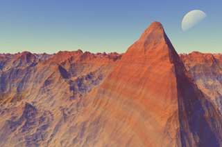
A fractal landscape created by Professor Ken Musgrave (Copyright: Ken Musgrave).
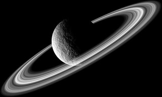
A fractal planet.
Further reading
The mathematics of fractals is discussed in a few fun web sites:
and in many books including:
- Fractals Everywhere, second edition, by Michael F Barnsley revised with the assistance of Hawley Rising III. Boston; London: Academic Press Professional, c1993
- Computers, Pattern, Chaos and Beauty: graphics from an unseen world by Clifford A Pickover. Stroud: Sutton 1990
- The Fractal Geometry of Nature by Benoit B Mandelbrot. San Francisco: W H Freeman, c1982
Some of the images and text in this article come from the following book:
- Fractal Geometry in Digital Imaging by Martin J Turner, Jonathan M Blackledge and Patrick R Andrews
- Charles Hermite
- David Hilbert
- Benoit B Mandelbrot
- J Henri Poincaré
- Claude Shannon
- Niels F H von Koch
- Karl T W Weierstrass
Comments
Anonymous
Fractals found in nature can prove to be random or exponentially symetrical but in the end can their pattern or lack of, lead us to better analysis
of disease; such as cancer or other aberrations in nature?
Jordn clepper
Yes because we can see how things work
Nervy
Hi!
I need a software to input a function which would display me a fractal - kind of like the program you used. What's the name of the program you used?