Extracting beauty from chaos

There are any number of sites on the World Wide Web dedicated to galleries of computer-generated fractal images. Pictures based on Lyapunov Exponent fractals, such as the one pictured above, are some of the most striking and unusual.
Like most fractal images, Lyapunov Exponent fractals are produced by iterating functions and observing the chaotic behaviour that may result.
In this article, we'll be exploring what Lyapunov exponents are, how you iterate functions, what "chaos" really is, and how you go about turning simple maths into marvellous images. There's also a companion article, Computing the Mandelbrot set by Andrew Williams, which looks at the technical details involved in writing a program to compute the Mandelbrot set.
What is iteration?
Even simple equations can produce complex behaviour when there is feedback in the system. For example, take a simple function like \begin{displaymath} f\left(x\right) = 4x\left(1-x\right) \end{displaymath} The graph of this function is just an upside-down parabola passing through the $(x,y)$ pairs $(0,0),\,(1/2,1),\,(1,0)$, as shown in the following figure:
Graph of the function f
The number $4$ in the definition of the function is there so that the graph of the function fits neatly into the unit box; in other words, if we apply the function to any number in the unit interval $0\le x\le1$, then we get another number in the unit interval. \par Now, pick a real number $x\left[0\right]$ between 0 and 1 (the "{initial condition}" or "{initial point}") and apply the function $f$ to this $x$ to get \begin{displaymath} x\left[1\right] = f\left(x\left[0\right]\right) = 4x\left[0\right]\left(1-x\left[0\right]\right) \end{displaymath} For example, suppose we choose $x[0]=0.3$; then we get $$ x\left[1\right] = f\left(x\left[0\right]\right) = 4(0.3)\left(1-0.3\right) = 0.84. $$ Now apply "{feedback}" to $x\left[1\right]$ by applying the function again to get $$ x\left[2\right] = f\left(x\left[1\right]\right) = f\left(f\left(x\left[0\right]\right)\right) $$ and keep repeating this process to get $$ x\left[3\right] = f\left(x\left[2\right]\right) = f\left(f\left(f\left(x\left[0\right]\right)\right)\right); $$ $$ x\left[4\right] = f\left(x\left[3\right]\right) = f\left(f\left(f\left(f\left(x\left[0\right]\right)\right)\right)\right), $$ and so on. \par So, for each number $n=0,1,2$,..., we put \begin{displaymath} x\left[n+1\right] = f\left(x\left[n\right]\right). \end{displaymath} \par This process is called "{iterating}" the function $f$ with the initial condition (or "{initial point}") $x\left[0\right]$. The sequence of numbers \begin{displaymath} x\left[0\right],\,x\left[1\right],\,x\left[2\right],\,x\left[3\right],... \end{displaymath} is called the "{orbit}" of the initial condition $x\left[0\right]$.
The butterfly effect
If we add a small error to the initial point $x\left[0\right]$, e.g. we look at \begin{displaymath} u\left[0\right] = x\left[0\right]+0.001 \end{displaymath} and then we look at the orbit $u\left[0\right],\,u\left[1\right],\,u\left[2\right],\,$... of $u\left[0\right]$, we might expect that the small error is not very important. \par However, it turns out that a function like the one above tends to {\em amplify small errors} until they become large, so the difference or "{error"} between the two orbits, i.e. the sequence \begin{displaymath} u\left[0\right]-x\left[0\right],\,u\left[1\right]-x\left[1\right],\,u\left[2\right]-x\left[2\right],\,... u\left[k\right]-x\left[k\right],\, ... \end{displaymath} tends to grow until it is as large as the numbers $x\left[k\right]$ themselves. \par The following diagrams illustrate this phenomenon: first, we show the orbit of an initial point in blue. We plot the points $x[k]$ (for $k=0,1,2$ etc.) against the step-number $k$: this is called a "time-series".
Orbit of an initial point
In the next picture, we compare this with the orbit of another close-by point, shown in red. In other words, we add a small error and look at what happens to the orbit:
Orbits of two initially close-by points
Notice that for the first few steps (on the left-hand side of the diagram), the orbits remain very close together and it seems that the small error hasn't made much difference. However, after just a few steps (toward the right-hand side of the diagram) the orbits begin to look completely different. The error has grown until the orbits are far apart.
The next picture shows the size of the error (i.e. the difference between the two orbits) at each step:
Error between the orbits
Notice how the error starts off very small, but after a few steps it has grown as large as the orbits themselves. This is like the noise in a radio transmission becoming as large as the signal itself and swamping it completely.
In fact, no matter how tiny we make the initial error, in most cases it will tend to be amplified until it grows large. This behaviour, where small errors tend to become amplified until they are as large as the "{signal}" itself, is called {\em sensitive dependence on initial conditions}. \par Another popular name for this phenomenon is the "{\em Butterfly Effect}", so-called because the idea is rather like the tiny flapping of a butterfly's wings becoming amplified until it causes a hurricane on the other side of the world. \par This is because the weather is sensitive to small errors in the same way that the function above is, so that - no matter how accurately we try to measure the weather right now (the temperature, humidity, etc.) - inevitably small errors in our measurements are amplified until they make our long-term weather forecasts unreliable. \par This effect is {\em one} of the hallmarks of "chaos": chaotic systems all have this feature (but not all sensitive systems are chaotic!) The other hallmarks of chaos are to do with periodic orbits ("{cycles}", where there is a repeating pattern in the orbit $x\left[0\right],x\left[1\right],$...) and "{mixing}" behaviour (like the kneading of dough, where orbits tend to get thoroughly "{mixed around}" throughout all the possible values). \par When all three hallmarks are present (sensitivity, periodic cycles and mixing), we have a phenomenon called "{chaos}". Unfortunately, Hollywood films have overused the word, so most people think that it means something altogether more wishy-washy, as opposed to a well-defined and precise mathematical term.Measuring sensitivity: The Lyapunov Exponent
So, we see that when certain systems are iterated, small errors tend to be amplified. How can we measure how quickly this happens?
A quantity called the "Lyapunov Exponent" (after its inventor, Alexander M. Lyapunov, 1857-1918) is used to measure the extent to which ever-smaller "infinitesimal" errors are amplified. In other words, the Lyapunov Exponent measures how sensitive a system is to errors.
Growth of small errors
Remember that we begin with a small initial error. Let's call this $E\left[0\right]$. So, we begin with \begin{displaymath} u\left[0\right] = x\left[0\right] + E\left[0\right] \end{displaymath} i.e. initial condition $x\left[0\right]$ and error $E\left[0\right]$. Then we compare the "{exact}" orbit $x[0],\,x[1],\,x[2],\,$... against the orbit with the error $u\left[0\right],\,u\left[1\right],\,u\left[2\right],\,$... and see how the difference between them grows. \par In other words, we look at the sequence of errors: \begin{eqnarray*} E\left[0\right]& = u\left[0\right]-x\left[0\right],\\ E\left[1\right]& = u\left[1\right]-x\left[1\right],\\ E\left[2\right]& = u\left[2\right]-x\left[2\right],\\ ... & \end{eqnarray*} \par The following picture demonstrates how an initial error $E[0]$ grows to give the error $E[1]$ at the next step for the function $f$ described above:
Growth of an initial error
To see how much the error is amplified at each iteration step $k$, we compute \begin{displaymath} \left| \frac{E\left[k+1\right]}{E\left[k\right]} \right| \end{displaymath} i.e. we see how big the next error $E\left[k+1\right]$ is, in comparison with the current error $E\left[k\right]$. (For example, if the next error were twice as big as the current one, then the expression above would have the value $2$.) \par After $n$ steps, the initial error $E\left[0\right]$ has been amplified by a factor of: \begin{displaymath} \left|\frac{E\left[n\right]}{E\left[0\right]}\right| = \left|\frac{E\left[n\right]}{E\left[n-1\right]}\right| . \left|\frac{E\left[n-1\right]}{E\left[n-2\right]}\right| . \,{\ldots}\, . \left|\frac{E\left[1\right]}{E\left[0\right]}\right| \end{displaymath} \par Now, suppose we had instead just looked at the simple linear function \begin{displaymath} g\left(x\right) = cx, \end{displaymath} where $c$ is some constant greater than 1. Then any error is simply magnified by $c$ at each iteration: \begin{eqnarray*} g\left(x+E\right) & = c\left(x+E\right) \\ \, & = cx + cE \\ \, & = g\left(x\right)+cE; \\ g\left(g\left(x\right)+cE\right) & = c\left(g\left(x\right)+cE\right) \\ \, & = cg\left(x\right)+\left(c^2\right)E \\ \, & = g\left(g\left(x\right)\right)+\left(c^2\right)E, \end{eqnarray*} so that after $n$ steps, the initial error has been magnified by \begin{displaymath} \left| \frac{E\left[n\right]}{E\left[0\right]} \right| = c^n \end{displaymath} (Note that if $c$ were less than 1, the error would actually be decreased rather than increased.) \par If we want to find out what the value of $c$ is for such a linear function $g$, we have \begin{displaymath} \ln\left(c\right) = \frac{1}{n}\ln\left(\left|\frac{E\left[n\right]}{E\left[0\right]}\right|\right) \end{displaymath} This is the idea behind the Lyapunov exponent: we take a {\em general} function $f$ and use this same formula to see how much small errors tend to be magnified. We take more and more iterates (larger and larger $n$) and calculate the corresponding values for $c$. If, as we let $n$ grow larger and larger, these values settle down to a constant, then this suggests that the error tends to grow on average like $c^n$. \par Taking the logarithm turns a product into a sum: \begin{eqnarray*} \frac{1}{n}\ln\left(\left|\frac{E\left[n\right]}{E\left[0\right]}\right|\right) &= \frac{1}{n}\ln\left(\left|\frac{E\left[n\right]}{E\left[n-1\right]}\right|. \left|\frac{E\left[n-1\right]}{E\left[n-2\right]}\right|.\,{\ldots}\,.\left| \frac{E\left[1\right]}{E\left[0\right]}\right|\right) \\ &= \left(\frac{1}{n}\right) \sum\limits_{k=1}^{k=n}\ln\left(\left| \frac{E\left[k\right]}{E\left[k-1\right]}\right|\right) \end{eqnarray*} \par The Lyapunov Exponent is defined to be the limiting value of the above quantity as the initial error $E\left[0\right]$ is made ever smaller-and-smaller, and the number of iterations $n$ is sent to infinity.
Lyapunov exponent of a differentiable function
\par Notice that \begin{displaymath} E\left[k\right] = f\left( x\left[k-1\right] + E\left[k-1\right] \right) - f\left( x\left[k-1\right] \right) \end{displaymath} so that \begin{displaymath} \frac{E\left[k\right]}{E\left[k-1\right]} = \frac{f\left(x\left[k-1\right]+E\left[k-1\right]\right) - f\left(x\left[k-1\right]\right)}{E\left[k-1\right]} \end{displaymath} \par Now, suppose that the function $f$ is smooth (i.e. we can differentiate it to get $f\prime\left(x\right)$). In this case, you should notice that the expression on the right-hand side looks familiar! Let's rewrite it like this (put ${h = E\left[k-1\right]}$ and ${x = x\left[k-1\right]}$): \begin{displaymath} \frac{E\left[k\right]}{E\left[k-1\right]} = \frac{f\left(x+h\right) - f\left(x\right)}{h} \end{displaymath} \par If we let $h$ go to zero, then this is just the expression for the derivative! So, as $h$ tends to zero we have: \begin{displaymath} \frac{E\left[k\right]}{E\left[k-1\right]} \rightarrow f\prime\left(x\left[k-1\right]\right) \end{displaymath} \par Thus we have \begin{eqnarray*} \left(\frac{1}{n}\right)\ln\left(\left|\frac{E\left[n\right]}{E\left[0\right]}\right|\right) &= \left(\frac{1}{n}\right) \sum\limits_{k=1}^{k=n} \ln\left(\left| \frac{E\left[k\right]}{E\left[k-1\right]}\right|\right) \\ &= \frac{1}{n} \sum\limits_{k=1}^{k=n} \ln\left(\,\left|\, f\prime\left(x\left[k-1\right]\right)\,\right|\,\right) \end{eqnarray} \par Finally, letting $n$ go to infinity (i.e. looking at more and more iterates), we obtain a formula for the Lyapunov Exponent of a differentiable function $f$: \begin{displaymath} \lambda\left(x\left[0\right]\right) = \lim\limits_{n \rightarrow \infty} \left(\frac{1}{n}\right) \sum\limits_{k=1}^{k=n} \ln\left(\,\left|\,f\prime\left(x\left[k-1\right]\right)\right\,|\,\right). \end{displaymath} \par If this number is positive, then this means that small errors in the initial condition $x\left[0\right]$ will tend to be magnified, and the system is showing sensitivity. (Remember that sensitivity is one of the three hallmarks of chaos.) If this number is negative, then small errors tend to be reduced, and the system is showing stability. \par So, the Lyapunov exponent gives us a way to measure the stability of our system.Order and Chaos in the same system
Even some very simple systems are capable of showing {\em both} orderly and chaotic behaviour. \par These systems may make transitions (called "{bifurcations}") from one type of behaviour to another, as some parameter is varied, rather like tuning-in to different radio stations by turning the dial on a radio. \par For example, remember our function \begin{displaymath} f\left(x\right) = 4x\left(1-x\right) \end{displaymath} whose graph was a parabola through $(x,y)=(0,0)$, $(1/2,1)$, and $(1,0)$. We can add a parameter $p$ to let us move the height of the parabola up and down: \begin{displaymath} f_{p}\left(x\right) = (4p)\,x\left(1-x\right) \end{displaymath} \par For a fixed number $p$ (with magnitude between 0 and 1) the graph of $f_{p}$ against $x$ is a parabola still passing through $(0,0)$ and $(1,0)$, but now having its "{top}" (turning point) at $(1/2,p)$, as shown in the following picture:
Graph of function with a parameter p
You can think of the parameter $p$ as being like the radio tuning dial: adjusting the value of $p$ moves the top of the parabola up and down smoothly, but as we will soon see the behaviour of the function can change suddenly. When tuning a radio, you sometimes happen to hit the right wavelength and hear a different radio station. In the same way, when the value of $p$ (the tuning dial) passes certain special values, the behaviour of orbits can change suddenly. \par There is a web page where you can experiment interactively with changing the value of the parabola and the position of the initial point $x[0]$: see Further Reading for details.
Plotting the stability
One idea to help us understand the way that the behaviour changes (as we change the parameter) is to plot the value of the Lyapunov exponent (for some chosen initial point $x\left[0\right]$) against the parameter $p$. This will let us estimate how the stability of our system changes as $p$ changes. \par The following diagram shows a plot of the calculated Lyapunov exponent (using the starting point $x[0]=1/2$) against the parameter $p$.
Lyapunov exponent vs. parameter
Notice the large negative spikes pointing downward. In reality, these spikes in the graph go off to minus infinity, showing that the behaviour of the function is incredibly stable at those parameter values. Remember that we have calculated an estimate of the logarithm of the error-multiplier: if this value is very large and negative, then the error-multiplier is very small, which indicates that errors tend to vanish away and the orbit of the system is super-stable.
Between the spikes, the graph touches the $p$-axis (so that the Lyapunov exponent is zero): this indicates that these parameters give an orbit which is on the edge of stable and unstable behaviour. It is here that sudden changes (bifurcations) in the behaviour of orbits take place.
Notice that the graph stays below zero until it reaches a point near the right hand side of the plot: this is where sensitivity first appears. As the graph rises above the axis, this means that the Lyapunov exponent is positive so that errors tend to be magnified. Even so, in this right-hand region there are still spikes where super-stable orbits appear.
There is much complicated structure in this diagram and even a simple one-parameter family of functions (like our parabola functions) still holds mysteries for mathematical research. There are also features of this plot that are universal, that is to say that we see them even when we look at very complicated functions, rather than our simple example; looking at simple situations in mathematics can sometimes throw light on more complicated ones.
Lyapunov-exponent pictures
To make a two-dimensional picture, we look at functions with {\em two} parameters (say $p$ and $q$), rather than just one. Then we use a colour to represent the Lyapunov exponent for each choice of the parameters $(p,q)$ in some rectangle. \par Conveniently, we can put these two-parameter functions together from a pair of one-parameter functions. For example, we can simply use the parabola function above. For numbers $p$ and $q$ we consider the functions: \begin{eqnarray*} P\left(x\right) &= (4p)\,x\left(1-x\right) \\ Q\left(x\right) &= (4q)\,x\left(1-x\right) \end{eqnarray*} \par Then, to make a single function, we combine them in some way. One way to do this is to apply them, one after the other, in some order. For example, we might apply $P$ first, then $Q$. So we would make our function $f$ from: \begin{displaymath} f\left(x\right) = Q\left(P\left(x\right)\right) \end{displaymath} (i.e. we are alternating between $P$ and $Q$) and we then iterate it as usual. (This means that, for example, $f(f(f\left(x\right)))\ = Q(P(Q(P(Q(P\left(x\right))))))$.) Or, we might choose \begin{displaymath} f\left(x\right) = Q(P(P(P(Q(P(Q\left(x\right))))))) \end{displaymath} or any other sequence of the functions $P$ and $Q$. Once we have decided what sequence of $P$ and $Q$ to use - let's choose $Q(P(x))$ - we keep it fixed from now on. \par Next, we work out the Lyapunov exponent for parameters $(p,q)$ in a grid. We're going to build our picture one dot (pixel) at a time. \par For each $(p,q)$ we take the initial point $x\left[0\right]=1/2$ and iterate $f$ to estimate the Lyapunov exponent, using the Chain Rule of differentiation to see that \begin{displaymath} f\prime\left(x\right) = \left(Q\prime\left(P\left(x\right)\right) \right).P\prime\left(x\right) \end{displaymath} and so we calculate the numbers \begin{displaymath} \ln\left|f\prime\left(x\left[k-1\right]\right)\right| \end{displaymath} for $k$ from $1$ up to some $n$, and average them. This gives us an estimate of the Lyapunov Exponent. (Choosing a larger value for $n$ generally gives a better estimate, but choosing $n$ too large means that a computer program will take a very long time to do the calculation for each point $(p,q)$.) \par We then colour the point corresponding to $(p,q)$ in our image, depending on the value that we estimated for the Lyapunov exponent. For example, we might choose dark reds for positive Lyapunov Exponents and Yellows for negative values, etc. We can choose a smoothly-spread range of colours when producing our pictures.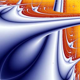
Part of the Lyapunov exponent picture for the QP sequence of maps
Understanding the pictures
Another Lyapunov Exponent picture
The sharply-defined curves which sometimes appear in these pictures correspond to very large negative Lyapunov exponents (meaning that the system is very stable, in fact "super"-stable, and errors tend to vanish away).
The background regions indicate positive exponents (where the system is sensitive, i.e. small errors tend to grow, and may be chaotic).
The presence of regions that appear to "cross over" each other reveals that there are two or more different types of behaviour that are "competing" with each other (in fact, these are competing "{attractors}") - different behaviours "win" the competition for different values of the parameters $p$ and $q$, so we see what look like different shapes crossing over each other. \par There are also repeating patterns and progressions of shapes, revealing lots of structure that would be difficult to guess just from looking at the simple equations used to generate the pictures. By visualising such structures and seeking to understand them, we can make progress in understanding the behaviour of more complicated models of systems in the real world. The beauty of these, and other, fractal images is an invitation to try and understand such patterns.Further Reading
Iteration of the logistic map:
If your browser can handle JAVA programs, then you can play with changing the height of the parabola and the position of the initial point $x[0]$ (see Order and Chaos in the same system) by looking at the web page Iteration of the Logistic Map.
Companion Article
- Computing the Mandelbrot set in this issue.
Other PASS Maths articles on fractals:
About the author

Andy Burbanks took a BSc in Mathematics and Computation at the University of Loughborough, and stayed on to do a PhD in Mathematics, during which time he developed an interest in mathematical artwork as a hobby.
He then spent a year as a mathematical artist, working with Bristol-based sculptor Simon Thomas (see The art of numbers in Issue 8).
He is currently doing research in dynamical systems in the Pure Maths Department at Cambridge University.
In addition to his research work, Andy is currently designing mathematical posters for the World Mathematical Year 2000's Posters in the London Underground project.
Comments
Anonymous
Hi,
If we let h tend to 0, then wouldnt f(x +h) - f(x)/h also tend toward 0? I dont understand how that equation is the equation of the derivative of the function f.
Marianne
When h tends to 0 both the numerator and the denominator of (f(x+h)-f(x))/h tend to 0. This does not mean that the whole expression tends to 0. As an example take f(x)=2x. Then (f(x+h)-f(x))/h=(2(x+h)-2x)/h = 2h/h = 2.
Girija Nair-Hart
First of all 0/0 is not equal to Zero.
It is 'indeterminate'. For example, think about 5*0/0, 10*0/5*o....
If there is a way to remove the 'thing' that is causing the 0's in the numerator and the denominator you will be able to find the 'vale' of the indeterminate form
vissinger
I don't understand the graph. If x[0]=1/2, then f'(x[0])=0, and ln(|f'(x[0])|)=ln(0)=- infinity. So for x[0]=1/2 Lyapunov exponent should be - infinity for all values of p.