In the light of recent events, it may appear that attempting to model the behaviour of financial markets is an impossible task. However, there are mathematical models of financial processes that, when applied correctly, have proved remarkably effective. In this article we look at one of these, a simple model for option pricing, and see how it takes us on the road to the famous Black-Scholes equation of financial mathematics, which won its discoverers the 1997 Nobel Prize in Economics.

Reckless trading of derivatives can cause huge losses.

In the world of business, companies would like to eliminate as much of their risk as possible. One of the ways of doing this is through buying financial products called derivatives. These products can be thought of as insurance policies: if a company buys one of these derivative products today, they can make sure that they are not exposed to certain risks in the future. These derivatives can also be traded in their own right; indeed, this trading has the potential to lose, as well as make, huge amounts of money.

As an example of a derivative, think of an airline selling a ticket today for a flight in a year's time. Fuel is one of the biggest costs of an airline, so it does not want to find that the price paid by the customer does not even cover the fuel in a year's time. A good way of avoiding this risk would be for the airline to enter into a forward contract, a type of derivative, which sets the price the airline will pay for fuel in one year's time. Of course, there is the chance that fuel prices could fall, in which case the price agreed in the forward contract may well be much higher than the price that the company would have paid if it had simply waited a year and bought the fuel then. However, most companies will prefer to get rid of as much risk as they can, which explains why derivatives are so useful for them.

Options

Of course, if a bank sells a derivative, it must know how much it should sell it for, and this is where the mathematicians come in. Suppose there is an asset whose price in the future is unknown. We will call this asset the stock (aka share), although the analysis we present would work for other assets, too. We will assume that the asset does not produce any dividends, that is, we don't receive anything for holding the asset. (This is a simplification, but it makes the analysis simpler and we could deal with dividends if we wanted to.) A derivative is then an asset whose price depends on the behaviour of the underlying stock. Throughout this article, we will look at a derivative called a European call. This is a contract which gives the holder the right (but not the obligation) to buy a stock at a fixed time in the future, for a fixed price. More specifically, the European call will specifya termination time, $T$, together with a strike price, $K$. The holder of the European call then has the right to buy the stock for price $K$ at time $T$. Of course, the holder will only buy the stock if $K$ is less than the price in the market. Thus, if the stock has price $S_T$ at time $T$, then the payoff of the European call will be $$\mbox{Payoff} = \left\{ \begin{array}{cc}S_T - K & \mbox{if this is greater than 0} \\ 0 & \mbox{otherwise}\end{array}.$$ A European call is a type of option, thus named because the holder has the choice to exercise it or not.

Pricing options: a simple model

What will the price of fuel be in a year's time?

There is a simple model, known as the binomial model, which gives us a way to price options. It is based on the same basic idea as the Black-Scholes model, which lies at the heart of financial mathematics and for which Myron Scholes and Robert Merton won the 1997 Nobel Prize in Economics (Fischer Black died two years before the award of the Nobel Prize).

We assume that there are just two assets: a bond and a stock. The bond is a riskless asset, which means that we know now what its value will be at the next time step. You can think of this bond as a bank account. A stock on the other hand is a risky asset, in the sense that we do not know its value in advance.

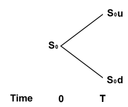
The stock price in a one-period binomial model.

We begin by looking at one time period. At the beginning of the period (time zero), the bond has price 1 and the stock has price $S_0$. At the end of the period (time $T$) the price of the bond will be $1+r$, where $r$ is the interest received over a time period of length $T$. In contrast, in this simplified model the risky asset can take one of two possible values: if the period is good, then the price will change by a known factor of $u$, so the stock price will increase to $S_0u$, whereas if the period is bad, the price will change by a known factor of $d$, so the stock will decrease in price to $S_0d$. We assume that the probability of a good period is $p$, although we will see later that (remarkably) this probability is not relevant when we come to work out the price of options.

A person in this model can hold as much as they like (positive or negative) of the stock or the bond. We also require the condition that $$d 1+r$, then everyone would borrow money (i.e. buy a negative amount of the bond) and use this money to buy the stock. At the end of the time period the value of the stock, even if it performed badly, would be more than what is owed on the bond. This strategy would guarantee to give a positive profit with no risk. A similar riskless strategy exists when $u

We now consider an option that has a payoff of $y_u$ if the stock goes up and $y_d$ if the stock goes down. How much would we be prepared to pay for this option? It turns out that there is a unique price because we can exactly replicate the payoff of the option.

Suppose that at time zero, we buy $x$ units of the bond and invest amount $z$ in the stock. At time $T$ our holding of bond is worth $x(1+r)$, and our holding in stock is worth $zu$ if the stock goes up and $zd$ otherwise. We are free to choose $x$ and $z$ however we like. In particular, we may choose them so that \begin{eqnarray*} x(1+r) & + & zu & = & y_u \\ x(1+r) & + & zd & = & y_d. \end{eqnarray*} If we choose such $x$ and $z$, then the value of our stock and bond at the end of the first period agrees exactly with that of the option. We can pay amount $x + z$ at time zero, and at the end of the first period we receive a payoff which exactly matches that of the option. The portfolio of stock and bond that replicates the payoff of the option is known as the replicating portfolio. The value of the option at time zero must be $x + z$, for if it traded at any other value, then there would be two entities (the replicating portfolio and the option) in our model that have the same payoff, yet cost different amounts. If this happened, everyone would buy one and sell the other in order to make a riskless profit. Hence, $x+z$ is the price of the option.

We can solve the two simultaneous equations above to show that $$z = \frac{y_u - y_d}{u-d} \;\;\;\; x=\frac{1}{1+r}\left(\frac{uy_d - dy_u}{u-d}\right).$$ The price of the option is now given by $$x+z = \frac{1}{1+r}\left( \left( \frac{1+r-d}{u-d}\right) y_u + \left(\frac{u-1-r}{u-d}\right) y_d\right).$$ To make things look simpler, we define $$q = \frac{1+r - d}{u-d}.$$ Then we can express the option price as $$C = \frac{1}{1+r}(qy_u + (1-q) y_d).$$

Equivalent probabilities

Rather surprisingly, the probability $p$ of a good period plays no part in this formula. If you're familiar with probability theory, then you might have thought that the expected value of the option payoff, a sort of average given by the formula $$py_u + (1-p)y_d$$ should appear in the formula for the option price. A similar expression does indeed appear, but with $p$ replaced by $q$, however $q$ is determined only by the interest rate $r$, and the possible changes in the stock price $u$ and $d$. The quantities $q$ and $1-q$ are accordingly termed equivalent probabilities. Remarkably, these equivalent probabilities suffice to determine the option price: the true probability of an up or a down jump is irrelevant.

On the road to Black-Scholes

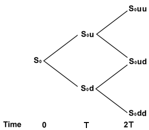
The stock price in a two-period binomial model.

Our model only lasts one time period, and we would like to extend it to a multi-period case. So let us suppose now that there are two periods, both of equal length $T$. In each period the stock can either go up or down, as shown in the diagram on the right. Now there are three possible outcomes for the value of the stock ($S_0uu$, $S_0du$ or $S_0dd$). We assume that the option now expires at the end of the second period and we let $y_{uu}$, $y_{ud}$, $y_{dd}$ be the value of the option in each of the three outcomes.

In order to price this option, first suppose that the stock went up during the first time period. Now consider how much stock and bond we should hold in order to replicate the payoff of the option at the expiry time. From our one-period model we know that if our portfolio of stocks and bonds is to be worth exactly $y_{uu}$ or $y_{ud}$ at expiry time, then at the beginning of the second time period it must be worth $$Y_u=\frac{1}{1+r}(qy_{uu}+(1-q)y_{du}).$$ Similarly, if the stock went down during the first interval, then our portfolio at the beginning of the second period should be worth $$Y_d=\frac{1}{1+r}(qy_{du}+(1-q)y_{dd}).$$ Applying our one-period model again, we see that for a portofolio to achieve values $Y_u$ or $Y_d$ after the first period, at time zero it needs to be worth $$C = \frac{1}{1+r}(qY_u + (1-q)Y_d).$$ Substituting the values for $Y_u$ and $Y_d$ we get $$C=\frac{1}{(1+r)^2}(q^2y_{uu}+2q(1-q)y_{ud}+(1-q)^2y_{dd}).$$ This is the price of a replicating portfolio and therefore the price of the option.

Using the same ideas, it is possible to extend this model to three, four, five, or any number of time periods. In fact, using some mathematical notation, it is possible to write down a general formula for $n$ periods $$C=\frac{1}{(1+r)^n} \sum_{k=0}^n {n \choose k} q^k (1-q)^{n-k}y_{u^k d^{n-k}}}.$$

The notation in this formula is explained here, but don't worry too much about the formula itself. The important point is that our technique of working backwards from the time of expiry works for any number of time periods. The brave reader might want to try and prove this result by induction.

Black-Scholes in the limit

You can work out the option price in a multi-period model by working backwards from the last period.

The binomial model is a very simple model for understanding the ideas behind option pricing. However, so far the stock price can only take finitely many values and furthermore can only move at discrete time points. Both of these features are somewhat undesirable, but there is a clever way around this problem. The basic idea is to divide the time to expiry of the option into $n$ equally-sized time periods and look at what happens to the model in the limit, as $n$ tends to infinity, in other words as the size of the time periods tends to zero. This will move our model from discrete time to continuous time.

The actual mathematics is a little too involved to be presented here (though the keen reader may want to look at it in our appendix). In fact, it is not necessary to go into it: the important point is that our simple model above can be turned into a single exact expression for pricing options. This is the famous Black-Scholes equation of financial mathematics. The only parameters it depends on are the strike price, $K$, the time to expiry, $T$, current stock price, $S_0$, the interest rate, $r$, and what is called the volatility. This parameter describes the variability of the stock price and has a precise mathematical definition.

The important message from our derivation is not so much the formula we end up with (shown here on the right), but rather the way in which we got it. We saw in our discrete time model how we were able to exactly replicate the payoff of our option by holding the correct amount of stock and bond. This then told us that the price of the option at time zero must be the amount that it costs to replicate the option.

The underlying idea in continuous time is exactly the same: we should pick our stock and bond so that they exactly match the payoff of the option at expiry time. Of course, since we are working in continuous time, the amount held in the stock and bond will need to be adjusted continuously, rather than at discrete time steps. However, the idea of replication is exactly the same.

Other options

The original Black-Scholes model assumed that stock price was a function of a random Brownian motion.

The original paper written by Black and Scholes in 1973 used the idea of replication to work out the price of the European call option, though their approach was a little different from the one taken here. They began directly with a continuous time model in which the stock price was a function of a Brownian motion: a random motion similar to the one you see when you let a particle float in a liquid or gas. Mathematically, Brownian motion is a stochastic process which satisfies certain properties. Black and Scholes' paper showed how the pricing of options can be transformed into a problem of solving partial differential equations with some given boundary conditions. Indeed, they were able to transform these partial differential equations and show that they were equivalent to solving the heat equation from physics. Unfortunately, the maths required to see the link with partial differential equation theory requires the machinery of stochastic calculus, which takes quite some effort to set up.

Although we have only shown how to price a European call option, we could use the same analysis to price any option whose payoff depends only on the terminal value of the stock. The Black-Scholes theory is indeed very general. However, there are also many other sorts of options, which don't fall under its remit. Pricing such exotic options creates many interesting problems in mathematics and keeps financial mathematicians in employment.

About the author

Angus Brown is a PhD student in the Statistical Laboratory at the University of Cambridge. Before starting his PhD, he completed his BA and Part III (both in maths) at Peterhouse, Cambridge.