Quantum computing: Some (not so) gruesome details

This article is part of our Information about information project, run in collaboration with FQXi. Click here to read other articles on quantum computing.

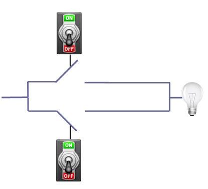
A current arriving from the left reaches the light bulb if one of the two gates is closed. Suppose that the two gates are closed when the corresponding switches are on and write 1 for a switch being on, 0 for a switch being off, and 1 or 0 for the bulb being on or off respectively. Then an input of two bits (corresponding to the switch positions) generates an output of one bit (corresponding to the state of the bulb).

In the previous article we gave you a rough idea of the physical processes quantum computers exploit in order to be more powerful than ordinary ones. Or would exploit, if it were possible to build large-scale quantum computers powerful enough to perform useful tasks. While this prospect is still some decades away, people do understand quite a lot of theory of quantum computation. Using the mathematics of quantum mechanics and logic, you can figure out what quantum algorithms can do even if you don't have an actual computer. In this article we look at one such algorithm in more detail: it's a simpler version of the one developed by Deutsch and Jozsa that is discussed in the previous article. You don't need to be familiar with the maths of quantum mechanics, as we'll guide you through the algorithm giving you as much information as you need.

A very important gate

An important fact in ordinary computer science is that any algorithm you might care to dream up can be implemented using a combination of a small collection of logic gates: as the name suggests, these are electrical circuits with gates in them, designed to take only one or two bits as input and produce a new bit as output. An example is the OR gate, shown on the right.

The same is true for quantum computing: a combination of a small number of quantum gates is enough to build any quantum algorithm — that has been proven mathematically. One of the most important ones is called the Hadamard gate, and it can actually be built in reality (see this article for a little more detail). When a Hadamard gate receives a qubit in state 0 as input, it returns a qubit as output that is in a superposition of 0 and 1 — it's both of them simultaneously.

It’s not just any superposition though. As we mentioned in the previous article, when you measure a system in superposition, it collapses and you only observe one of the possible outcomes. If we measure the output of the Hadamard gate after it’s received a qubit that’s a 0, there is a 50:50 chance of seeing a 0 or a 1. Physicists have a special way of writing this superposition:

$\frac{1}{\sqrt{2}} |0\rangle + \frac{1}{\sqrt{2}} |1\rangle .$

A qubit in superposition is like a switch being on and off at the same time.

The terms $|0\rangle$ and $|1\rangle$ stand for the qubit being a 0 or a 1 and the $+$ symbol indicates that we have a superposition of both possibilities. But why does each term come with a $1/\sqrt{2}$ rather than a $1/2,$ which corresponds to the probability of observing it?

The answer would take us deeper into the mysteries of quantum mechanics, so let's just say this: in ordinary life, we deal with probabilities, which are always positive numbers. The sum of the probabilities of alternative outcomes (such as seeing a 0 or seeing a 1) is always 1. In quantum mechanics there is a more general concept, called a probability amplitude, which is allowed to be a negative number (in fact, amplitudes are complex numbers). The amplitudes of alternative outcomes don't need to add up to 1, but the sum of their squares does. The coefficients in our expression above are amplitudes, and they satisfy this requirement:

$(1/\sqrt{2})^2 +(1/\sqrt{2})^2 = 1/2+1/2 =1.$

Amplitudes are related to probabilities through squaring: the probability of seeing a particular outcome when you make a measurement is the square of the absolute value of its amplitude. So in our example above, the amplitude $1/\sqrt{2}$ corresponds to the probability of $1/2,$ as required.

So much for feeding a qubit in state 0 into a Hadamard gate. When a qubit that is in state 1 passes through it, it is also put into a superposition of 0 and 1, but this time the amplitude of $|1\rangle$ is negative:

$\frac{1}{\sqrt{2}} |0\rangle - \frac{1}{\sqrt{2}} |1\rangle .$

How does this differ from the state we got from inputting a 0? The squares of the amplitudes are the same in each case, so measuring gives a 50:50 chance of seeing a 0 or a 1 in both cases. The difference lies in how the two states evolve over time and interact with other states or qubits. Probability amplitudes are complex numbers, which contain more information than just a single positive number. In some sense all the mystery of quantum mechanics, the weird phenomena like superposition that don’t chime with our experience of the world, is hidden in that extra information.

Interference

The Hadamard gate also gives us a good example of another phenomenon that’s important in quantum computing, called interference. To see how this works, let’s pass a $|0\rangle$ through the Hadamard gate to get the superposition

$\frac{1}{\sqrt{2}} |0\rangle + \frac{1}{\sqrt{2}} |1\rangle .$

What happens to this if we pass this through the Hadamard gate again? Luckily, nature has been kind in making the maths needed to work this out quite easy. We can muddle through even without a formal introduction: simply apply the formulae from above, which tell us what the gate does to a $|0\rangle$ and a $|1 \rangle ,$ to the individual components of the superposition. This gives

$\frac{1}{\sqrt{2}} \left(\frac{1}{\sqrt{2}} |0\rangle + \frac{1}{\sqrt{2}} |1\rangle \right) + \frac{1}{\sqrt{2}} \left(\frac{1}{\sqrt{2}} |0\rangle - \frac{1}{\sqrt{2}} |1\rangle \right).$

Multiplying out the brackets it’s easy to see that the $|1\rangle$ terms cancel out, leaving us with

$\frac{1}{2}|0\rangle + \frac{1}{2}|0\rangle = |0\rangle .$

The amplitude of $|0\rangle$ in this expression is $1,$ which means that if we measure the qubit now we will definitely see a $0$ .

Waves can interfere constructively, re-enforcing each other, or destructively, cancelling each other out.

Interference is exactly this cancellation or adding up of terms. There is destructive interference, where the coefficients of a term — $|1\rangle$ in our example — cancel out, so the term disappears. And there is also constructive interference, with coefficients adding up. This is what happened to the term $|0\rangle$ in our example. People often think of this in terms of waves, which can also interfere constructively or destructively (see here for an explanation).

Interference means that starting with $|0\rangle$ and applying the Hadamard gate twice gives you back the initial $|0\rangle :$

$|0\rangle \rightarrow \frac{1}{\sqrt{2}} |0\rangle + \frac{1}{\sqrt{2}} |1\rangle \rightarrow |0\rangle .$

You can convince yourself that the analogous thing happens when you start with a $|1\rangle :$

$|1\rangle \rightarrow \frac{1}{\sqrt{2}} |0\rangle - \frac{1}{\sqrt{2}} |1\rangle \rightarrow |1\rangle .$

An example

Now let’s return to the algorithm developed by Deutsch and Jozsa, which we used as an example in the previous article. The task to perform was to check whether a function that takes bit-strings of 0s and 1s as input is constant or balanced. Constant means that the function allocates the same value, 0 or 1, to all bit-strings. Balanced means that it allocates a 1 to exactly half of the bit strings and a 0 to the other half.

The simplest possible situation is when the bit-strings that form the input of the function are only one bit long. A constant function $f$ would be either:

$f(0) = 0 \mbox{ and } f(1)=0,$

$f(0) = 1 \mbox{ and } f(1)=1.$

And a balanced function would be either

$f(0) = 1 \mbox{ and } f(1)=0,$

$f(0) = 0 \mbox{ and } f(1)=1.$

If you are working with a classical computer, then a program that finds out whether the function is constant or balanced needs to look up the values of the function twice: once to check its value for $0$ and once to check it for $1.$ There just isn’t a quicker way of finding the answer to your question. What Deutsch and Jozsa showed in 1992 is that there’s a quantum algorithm which can look up the value of the function for both $0$ and $1$ simultaneously and then tell you whether the function is constant or balanced.

The general idea

The algorithm uses two basic facts. The first fact involves the superposition state

$\frac{1}{\sqrt{2}}|0\rangle - \frac{1}{\sqrt{2}} |1\rangle = \frac{|0\rangle - |1\rangle }{\sqrt{2}} .$

You can change this state into its negative simply by adding $1$ to each component, using binary addition, which means that $1+1$ is equal, not to $2$ , but to $0$ . This gives

$\frac{|0+1\rangle - |1+1\rangle }{\sqrt{2}} =\frac{|1\rangle - |0\rangle }{\sqrt{2}} = -\frac{|0\rangle - |1\rangle }{\sqrt{2}}.$

We’ll keep this in mind as a potential method for changing signs.

The second fact is the one we already saw above. That a Hadamard gate changes the superposition states

$\frac{|0\rangle + |1\rangle }{\sqrt{2}} \; \; \; \mbox{and}\; \; \; \frac{|0\rangle - |1\rangle }{\sqrt{2}}$

into $|0\rangle$ and $|1\rangle$ respectively.

Now suppose you are dealing with a similar superposition state, but with the signs of the two amplitudes determined by the values of the function $f$ . Let’s call this state $|\psi \rangle$ :

$|\psi \rangle = \frac{ (-1)^{f(0)}|0\rangle + (-1)^{f(1)} |1\rangle }{\sqrt{2}}.$

This means that the amplitude of $|0\rangle$ has a negative sign if $f(0)=1$ and a positive one of $f(0)=0.$ The same goes for the amplitude of $|1\rangle .$ A constant function would therefore give you

$|\psi \rangle = \pm {\frac{ |0\rangle + |1\rangle }{\sqrt{2}}}$

and a balanced function

$|\psi \rangle = \pm {\frac{ |0\rangle - |1\rangle }{\sqrt{2}}}.$

When we apply the Hadamard gate to the state $|\psi \rangle ,$ the signs simply pass through the process. A constant function results in either a $|0\rangle$ or a $-|0\rangle .$ Whichever it is, when we make a measurement, we will definitely see a $0.$

A balanced function results in either a $|1\rangle$ or a $-|1\rangle .$ Whichever it is, when we make a measurement, we will definitely see a $1.$

Therefore, if we can produce the state $|\psi \rangle$ somehow, the Hadamard gate will give us the answer to our question, whether $f$ is constant or balanced, with certainty.

The algorithm

Now let’s put all this together and see how the algorithm works. Since it is based on two facts, you might not be surprised that it uses two qubits. First note that to answer the question of whether $f$ is constant or balanced, whether we do this classically or using quantum computing, we obviously need to assume that the computer has some method for "looking up", or computing, values of $f$ : given an $0$ or a $1$ it needs to be able to find out what $f(0)$ or $f(1)$ is. This is something we take as a given, which is why we call this method a black box: we know what it does, but we don’t care how it does it.

We can equally-well assume that we have a black box that works with two pieces of information, an input register and an output register. In the case of classical bits, given an input register set to $i$ (which is a $0$ or a $1$ ) and an output register set to $j,$ (also a $0$ or a $1$ ) the black box finds $f(i)$ and adds it to $j,$ giving $i, j+f(i)$ as the result. The addition here is again binary (and hints towards our first fact above). Our box is just another way of telling us what $f(i)$ is, and in terms of answering our question, this doesn’t make a difference: we would still need to use the box twice to decide if the function is constant or balanced.

In the quantum context the registers are qubits and the black box is a quantum gate which transforms the two-bit system made up of $|i\rangle$ and $|j\rangle$ (where $i$ and $j$ are $0$ or $1$ ) into $|i\rangle$ and $|j+f(i)\rangle .$

And here comes the trick. To produce the state $\psi$ we apply the box with input register

$\frac{|0\rangle + |1\rangle }{\sqrt{2}}$

and with output register

$\frac{|0\rangle - |1\rangle }{\sqrt{2}}.$

The input register will be transformed into $\psi .$ The transformation involves nothing more than potential sign switches (depending on $f$ ) and these will be performed with the help of the output register, which, as fact one above tells us, is capable of performing this task.

Once $|\psi \rangle$ has been produced in this way (with one use of he black box) we simply use the Hadamard gate to find out whether $f$ is constant or balanced.

The calculation

To show that our box really does the right thing, we make use of the very convenient fact that our two-bit system can be mathematically represented as a product:

$\left(\frac{|0\rangle + |1\rangle }{\sqrt{2}}\right)\left(\frac{|0\rangle - |1\rangle }{\sqrt{2}}\right),$

which can be rewritten as

$\begin{equation} \frac{1}{\sqrt{2}} \Bigg( |0\rangle \frac{\left(|0\rangle - |1\rangle \right)}{\sqrt{2}} + |1\rangle \frac{\left(|0\rangle - |1\rangle \right)}{\sqrt{2}}\Bigg). \end{equation}$

(1)

To see what the black box does to the term

$|0\rangle \frac{\left(|0\rangle -|1\rangle \right)}{\sqrt{2}}$

we simply see what it does to each component of the superposition $|0\rangle - |1\rangle .$ This gives:

$|0\rangle \frac{\left(|0+f(0)\rangle -|1+f(0)\rangle \right)}{\sqrt{2}}.$

When $f(0)=0,$ this is just

$|0\rangle \frac{\left(|0\rangle -|1\rangle \right)}{\sqrt{2}}.$

But when $f(0)=1,$ fact one above tells us that we have

$|0\rangle \frac{-\left(|0\rangle -|1\rangle \right)}{\sqrt{2}}.$

Putting this together (passing the potential sign change through the expression) we have

$\begin{equation} (-1)^{f(0)}|0\rangle \frac{\left(|0\rangle - |1\rangle \right)}{\sqrt{2}}.\end{equation}$

(2)

Similarly, the black box turns the term

$|1\rangle \frac{\left(|0\rangle -|1\rangle \right)}{\sqrt{2}}$

into

$\begin{equation} (-1)^{f(1)}|1\rangle \frac{\left(|0\rangle - |1\rangle \right)}{\sqrt{2}}.\end{equation}$

(3)

Substituting (2) and (3) back into (1) gives

	$\displaystyle$	$\displaystyle \frac{1}{\sqrt{2}} \Bigg( (-1)^{f(0)}\|0\rangle \frac{\left(\|0 \rangle - \|1\rangle \right)}{\sqrt{2}}+(-1)^{f(1)}\|1\rangle \frac{\left(\|0 \rangle - \|1\rangle \right)}{\sqrt{2}}\Bigg)$
	$\displaystyle =$	$\displaystyle \Bigg(\frac{(-1)^{f(0)}\|0\rangle + (-1)^{f(1)}\|1\rangle }{\sqrt{2}}\Bigg)\Bigg( \frac{\|0 \rangle - \|1\rangle }{\sqrt{2}}\Bigg)$
	$\displaystyle =$	$\displaystyle \|\psi \rangle \frac{\left( \|0 \rangle - \|1\rangle \right)}{\sqrt{2}}.$

Here is the state $|\psi \rangle$ we were after!

Deutsch's and Jozsa's algorithm was a breakthrough because it was the first quantum algorithm that was provably better than a classical one: it needed only one shot of looking at the function values (simultaneously for 0 and 1) rather than two. They later generalised the algorithm to work for functions that don't take just 0s and 1s as input, but strings of them (see the previous article). They proved that in this case the quantum algorithm is exponentially faster than its classical counterpart.

That's all very exciting, but is it any use? The problem the Deutsch-Jozsa algorithm solves isn't particularly useful in the real world. What other tasks can quantum perform better than classical ones? And how far away are we from having fully functional quantum computers? To find out, read the following articles:

About this article

Richard Jozsa

Marianne Freiberger is Editor of Plus. She would like to thank Richard Jozsa, Leigh Trapnell Professor of Quantum Physics at the University of Cambridge, for his extremely helpful, very patient and generally invaluable explanations.

Comments

The Article

The diagram at the start of this article is misleading. Given that the circuit is open unless both switches are closed the initial statement appears to be incorrect.

I thought this at first

I thought this at first glance as well, but it should be assumed that both sides of the shown circuit connect outside of the shown portion. Since the two switches are in parallel, if either is closed the circuit will be completed.

switch diagram

It's just an OR gate in classical computing. Either path can light up the bulb.
An or gate in classical computing does the same thing.

Using a lot of photons instead of individual qubits seems better

So as I understand this, a group of single qubits will never give as much detail as we need, better to make a large string of individually entangled pair photons, then you can read a lot more data points of one equation, using just one entanglement for each measurement.

Binary Addition

In what way does the result of the binary addition of 1+1 =0? Are we referring to the digit value and the remaining information is sloughed off or something? Very hung up on that.