

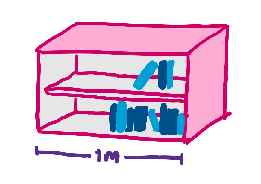
We use measurements all the time in our daily life. The length of this bookshelf is 1 metre, the volume of that swimming pool is 30,000 litres. In maths, we often take measurements as well. On the real line, the length of the interval [0,1] is 1, and in 3D space, the volume of a cube with side length 1 is 1. Makes sense, right?
Mathematicians, however, always like to ask pesky questions to test the limits of their definitions. Does everything have a length? What, for example, should the length of the set of rational numbers (that is, numbers such as 3/5 or 14/17 that can be written as fractions) between 0 and 1 be?
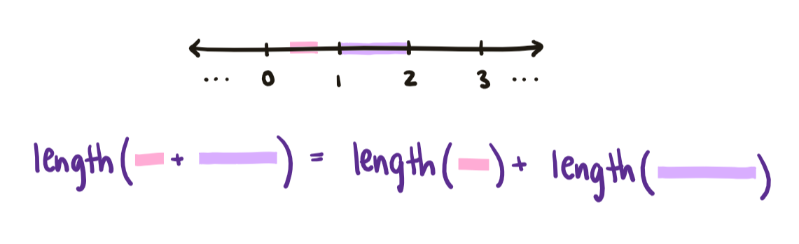
To answer such questions, we need a way to describe what exactly length, area, and volume mean mathematically. Let’s focus on length to begin with. Length is a function: it takes in objects (such as bookshelves or intervals) and outputs their length, a nonnegative real number. Additionally, the total length of two non-overlapping things is always the sum of their individual lengths. For example, the length of two bookshelves lined up end-to-end is the sum of their lengths. Similarly, the total length of two non-overlapping intervals is the sum of their lengths.
We can extend this observation slightly, and impose that the total length of countably infinite many things is also always the sum of their individual lengths. For example, the total length of the intervals $[0,\frac{1}{2}], [\frac{1}{2}, \frac{3}{4}], [\frac{3}{4}, \frac{7}{8}],\dots$ should be 1. This is because the sum ½ + ¼ + ⅛ + … , despite having infinitely many terms, converges to the number 1: as you add more and more terms, it gets closer and closer to 1 but never exceeds it.
These are really the two key things we need to know about length:
- It is a function which takes in measurable objects and outputs their length, a nonnegative real number
- It is countably additive: the total length of countably infinite many things is the sum of their individual lengths.
Notice that area and volume should also have these two properties. In general, we call such functions measures. That is, a measure is a function which takes in objects from some allowed set and outputs nonnegative real numbers in a countably additive way. Whew!
With this formalism in hand, we can begin to answer those pesky length questions we couldn’t answer before. How long is the set of rational numbers between 0 and 1? We know that there are infinitely many rational numbers between 0 and 1; but importantly, they are only countably infinite. In comparison to the uncountably many real numbers between 0 and 1, the rational numbers are just a drop in the ocean. We expect our notion of length to reflect this, and indeed it does. The length of each individual real number must be 0 — otherwise the interval, which contains infinitely many real numbers, would be infinitely long. Hence the length of the set of rational numbers between 0 and 1 must be the countable sum 0 + 0 + … + 0 = 0!
Does every subset of the real line have a length? Well, that’s a story for another time…
Where do measures come from?
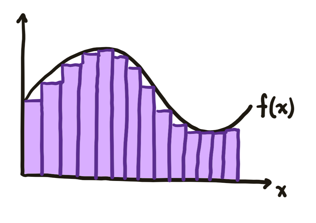
Historically, measures were initially formalised in order to construct a more powerful definition of integration. We can think of integration as the problem of measuring the area under the graph of a function. Before the formalisation of measure, the primary tool mathematicians had for measuring the area of unknown shapes was to approximate those shapes with simpler shapes, such as rectangles, whose area was known. And so, Bernhard Riemann had constructed his theory of integration by approximating the graphs of functions with rectangles. Each rectangle had a base which was an interval of the real line, and by making the intervals smaller and smaller he got a better and better approximation of the area under the function graph.
Our modern notion of measure was formalised by mathematician Henri Lebesgue in his 1902 doctoral thesis titled Integral, Length, Area. Armed with his new formalism, Lebesgue no longer had to restrict himself to measuring functions using rectangles whose bases were intervals. Instead, he could enlarge his measuring tool to rectangles whose bases were measurable sets - that is, any set which has been assigned a measure. For example, we could have a rectangle whose base was the set of rational numbers between 0 and 1. With these more powerful measuring tools, he arrived at a much more powerful and natural theory of integration, which is still the primary theory of integration today.
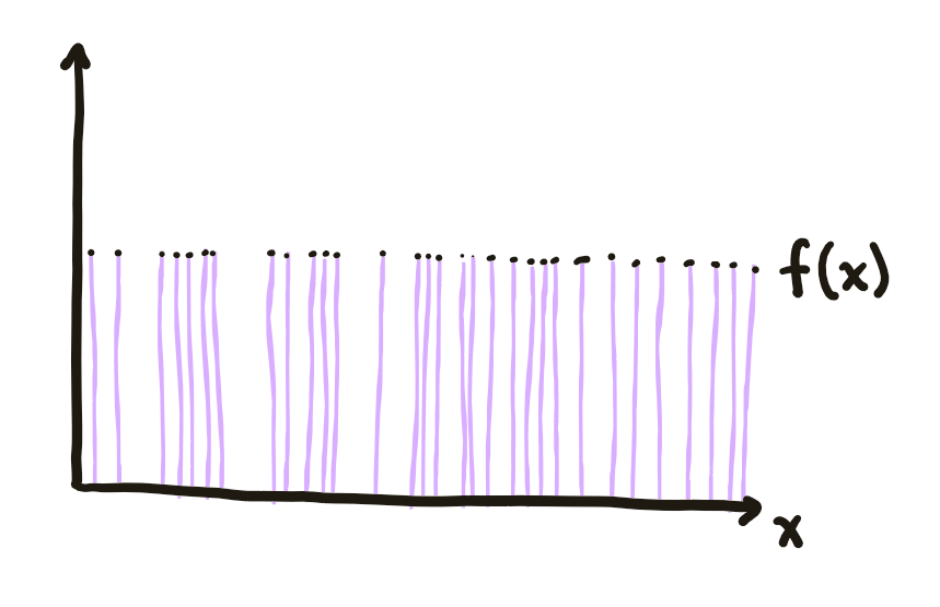
The Lebesgue integral allows us to integrate functions such as the Dirichlet function, which is 1 at every rational number and 0 everywhere else.
Measures and probability
By the 1930s, measures had found a natural home in the theory of probability. Suppose that we have bought a handful of lottery tickets, and are waiting for the winning numbers to be called. The set of all the lottery tickets is our probability space. In our hand we have some subset of all the possible tickets. We can think of the probability that one of our tickets is the winner as the measure of our hand of tickets. This is the formalism that modern probability theory is built on: in the same way that length assigns a measure to subsets of the line, probability is a way of assigning a measure to subsets of possible outcomes.
Here’s one way in which the concept of measure helps us be more precise when talking about probabilities. What does it mean to pick a random integer? We might say that it means to pick an integer in a way such that every integer is equally likely to be picked. But in fact this is impossible!
Suppose we tried by letting $p$ be the probability that any individual integer is picked. If we picked $p > 0$ to be strictly positive, then the probability we picked an integer between 1 and $N$ would be $Np$. But we can always find an $N$ such that this probability is bigger than 1, a contradiction.
Instead suppose we picked $p$ to be exactly 0. Since probability is a measure, it is countably additive. That is, the probability of picking any one of countably many integers is the sum of the probabilities of picking each integer individually. Hence if we pick $p$ to be 0, the probability we pick any integer at all is 0 + 0 + … = 0! This is also a contradiction since we always must pick some integer: the sum of all the probabilities in a probability space must always be equal to 1. Since $p$ can be neither 0 nor strictly positive, there is no way to assign the same probability $p$ to all the integers.
For more about measures
Read more about measures, integrals, and non-measurable sets here: Measure for Measure.
Read more about the axioms of probability at Maths in a minute: The axioms of probability theory.
And as an application to fractals: the Hausdorff measure allows us to talk about the volume of fractional-dimension objects. Read more at How to compute the dimension of a fractal.