The making of the logarithm
Portrait of John Napier (1550-1617), dated 1616.
Tables of numbers related in a very similar way were first published in 1614 by the mathematician, physicist and astronomer John Napier in a paper called The construction of the wonderful canon of logarithms. Surprisingly, though, Napier had never even heard of the number e, nobody had at the time, and he wasn't really thinking about exponentiation either. When he inadvertently defined something very similar to the logarithm to base e, he did so by imagining points moving along lines!
One problem that was plaguing people at the time, especially astronomers, was arithmetic. Astronomical calculations required the multiplication and division of very large numbers, something that's pretty hard to do without a calculator. One way of making things easier is to think in terms of powers. As the rules of exponentiation tell us, to multiply two powers of 2, say $2^a \times 2^b$, you only need to add their exponents. To divide them, you simply subtract their exponents: $2^a \times 2^b = 2^{a+b}$ $\frac{2^a}{2^b} = 2^{a-b}.$ So a table telling you how to express large numbers as powers of 2, or of any other number, would help you simplify your calculations considerably. Given a number $N$ you would be looking for the number $L$ so that $$N=2^L.$$In other words, what you'd want are tables of logarithms to the base 2, or some other number.
In Napier's time, however, people were not used to thinking in terms of exponentiation. They didn't have the concept of a base and they didn't have our handy way of writing powers, using a little number at the top.
What they were aware of, though, since the time of Archimedes, was an interesting link between the sequence you get by starting with 2 and successive doubling (which we today recognise as the sequence of powers of 2):
2, 4, 8, 16, 32, 64, 128, … .
and the sequence of natural numbers
1, 2, 3, 4, 5, 6, 7, … .
The first sequence is called a geometric progression because successive numbers have the same ratio; 2. The latter is called an arithmetic progression because successive numbers have the same difference; 1.
People noticed that multiplying (or dividing) two numbers in the geometric progression corresponds to adding (or subtracting) the corresponding numbers in the arithmetic progression. (To us, these are just the laws of exponentiation again, as numbers in the geometric progression are powers of 2, and the numbers in the arithmetic progression are the corresponding exponents.) This seemed to offer a way of making calculations easier, as you could replace the harder operations in the geometric progression with easier ones in the arithmetic progression.
Napier wanted to produce a table that related numbers in a useful geometric progression to numbers in a corresponding arithmetic progression so that, as he wrote, "All multiplications, divisions and [...] extraction of roots are avoided," and replaced by "most easy additions, subtractions and divisions by 2."
It's the way he found the two sequences that is so intriguing. Imagine a point, call it $P$, moving along a finite line segment from a point $A$ to a point $B.$ It doesn't move at uniform speed, however, but slows down continually: its speed at any given moment is proportional to the distance still left to travel to the point $B$. The closer to $B$ the point gets, the slower it gets, so it will never actually reach $B$. If you measured the distance still left to travel to $B$ at regular time intervals, say every second, then the numbers you'd get would form a decreasing geometric progression: ratios between successive numbers would be equal, but unlike on our example above, they'd be smaller than 1.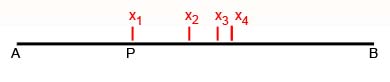
Today we would use calculus to work out Napier's logarithm. If you do this (see here to find out how), you will find that
$$\frac{x}{10^7} = \frac{1}{e}^{\left(\frac{y}{10^7}\right)},$$ where $x$ is the distance still to travel by $P$ and $y$ is the distance already travelled by $Q.$ This means that $\frac{y}{10^7}$ is the logarithm to base $1/e$ of $\frac{x}{10^7}$ — essentially that's what Napier's construction defines. But since calculus had not been invented in Napier's time, his table gave an approximation of this logarithm, relating $x$ and $y$ by the relationship $$\frac{x}{10^7} =\left(1-\frac{1}{10^7}\right)^y.$$ To see that this really is a good approximation, rewrite the expression as $$\frac{x}{10^7} = \left(1-\frac{1}{10^7}\right)^{10^7\left(\frac{y}{10^7}\right)}.$$ If you are familiar with the many beautiful properties of the number $e$, then you will know that for any real number $x$, $e^{x}$ is the limit as $n$ goes to infinity of $$\left(1+\frac{x}{n}\right)^{n}.$$ Taking $x=-1$ gives $$\lim_{n \rightarrow \infty}{\left(\left(1-\frac{1}{n}\right)^{n}\right)} = e^{-1}=\frac{1}{e}.$$ And since $10^7$ is a very large number, the number $$\left(1-\frac{1}{10^7}\right)^{10^7}$$ that appears as the base in Napier's logarithms is very close to the limit $\frac{1}{e}$. Therefore, since $$\frac{x}{10^7} = \left(1-\frac{1}{10^7}\right)^{10^7\left(\frac{y}{10^7}\right)},$$ $\frac{y}{10^7}$ is very close to the logarithm to base $\frac{1}{e}$ of $\frac{x}{10^7}$. That's why Napier's work is often counted as the first, albeit implicit, appearance of the number $e$ in mathematical history. And Napier is today credited with inventing the natural logarithm — without ever having heard of $e!$About the author
Marianne Freiberger is Editor of Plus.
Comments
Anonymous
Logarithms discovered by Napier in 1614 were based on sine tables with 0.9999999 just below sine 90 degrees as the base which is raised to successive powers. Initially the results are nearly equal to the shortfall from 1.0000000. It would be a very onerous task to raise these powers from sine 90 degrees down to sine 1 degree, but this would be helped by by sine 75 degrees equalling 0.9659258 being raised to the power of 10 and equalling sine 45 degrees which is 0.7070299. Without these tables of logarithms there would be no theory from Nicholas Mercator of the area under a symmetrical hyperbola equalling the log of the distance along the x axis, nor of Isaac Newton's reversion of the hyperbola formula to achieve the infinite series for the antilogarithm e. This year is the 400th anniversary of Napier's discovery which is not being properly commemorated largely because modern mathematicians have no idea how Napier achieved it. submitted by Peter L. Griffiths.
Anonymous
Napier and Regiomontanus before him knew the formulae for constructing sine and cosine tables. Basically this is sin2u equals 2sinu.cosu. This can be converted into sin2u equals 2sinu. (1-[sinu]^2)^0.5 ,so that if the sine of a particular angle is known then the cosine can be calculated, also the sine of half that angle can be calculated by quadratic equation. The sine of 75 degrees can therefore be calculated from bisecting sin30 degrees ( which is 1/2) to give the sine of 15 degrees which is the cosine of 75 degrees, from which the sine of 75 degrees can be calculated. submitted by Peter L. Griffiths.
Anonymous
Very few modern mathematicians have grasped that sine 75 degrees raised to the power of 10 equals sine 45 degrees. Napier's angles just below 90 degrees are incorrect. The arc sine of 0.9999999 is much closer to 89 39/40 degrees than it is to 89 59/60 degrees. This could explain why nobody seems to have attempted to list the corresponding arc cosines. submitted by Peter L. Griffiths. We can hardly blame school maths when the experts are so negligent.
Peter Norvig
Perhaps the reason that so few mathematicians "have grasped that sine 75 degrees raised to the power of 10 equals sine 45 degrees" is that sin(75 degrees) = (1 + sqrt(3))^10/32768, while sin(45 degrees) = sqrt(2)/2, which are different numbers (although they happen to agree to 3 decimal places).
richard1941
You are correct, according to my WP-35s calculator set to double precision. The difference is .00007688.... . I am still wondering how Napier did it. Something like bisection using square roots maybe?
Anonymous
In the Constructio paragraph 44, Napier rather obscurely states a formula for calculating the logarithms of sine 89 39/40 degrees down to log sine 75 degrees. This is 10^7 X (0.9999999)^5000s equals 10^7 - 5000s + 5/4 s^2. If s is 1, then we have an equality where the shortfall is about 3200. However if s is about 69, we have the log of sine 75 degrees. From log sine 75 degrees to log sine 45 degrees, sine 75 degrees raised to the power of 10 is sine 45 degrees. This power of 10 can be split up to measure the intervening logarithms. It is no use expecting modern mathematicians to know anything about this, submitted by Peter L. Griffiths.
Peter L. Griffiths
Napier recognised that the formula for the hyperbola 1/(1+x) = 1-x +x^2 - x^3....
could be converted into measuring the area under the hyperbola by integration, similar
to the conversion of the circumference of a circle 2PIr intothe area of the circle PIr^2.
S(1/1+x) = x - x^2/2 + x^3/3 - x^4/4.....
Multiplying both sides by 1/2 gives
1/2S(1/1+x) = x/2 - x^2/4 + x^3/6 -x^3/8.....
Napier very cleverly recognised that S(1/1+x) could be represented log(1 + x),
so that 1/2S(1/[1+x]) could be represented as 1/2 log(1 +x) or log (1 +x)^1/2.
In this way with x = 1, log2 = 1 - 1/2 + 1/3 - 1/4....= 0.693148
and log 2^1/2 = 1/2 - 1/4 + 1/6 -1/8.......= 0.346574.
Napier mentions amounts close to 0.693148 and 0.346574 in paragraphs 46-53
of the Constructio.
mathlover
Hi Peter,
Could you please post some images of the above derivations so that it would be clear. I am also interested to know the resources from which you have got this.
If you have any blog of your own let me know. Thank you
mathlover
Hi could you let me know the resources to study so that I can understand your comment. I have gone through the book invention of napier logarithm by hobson but couldn't get it. Can you explain me how logarithm were invented at the beginning of 16th century on trigonometric functions. A video tutorial would help a lot for the further generations to learn these inventions.
Anonymous
Hi,
Rigth after «you will find that», I'd put parentheses around 1/e instead of y/10^7.
Thanks for this very interesting article.
Anonymous
Further to my previous comments, I have come across an interesting approximate relationship which could have helped Napier in constructing his log tables. This is cos30 equals (cos15)^4. This seems approximately to apply to angles below 30 degrees, and in particular should be helpful in calculating the logarithms of cosines below 30 degrees and of sines of angles above 60 degrees that is sin60 equals (sin75)^4. submitted by Peter L. Griffiths.
Anonymous
One clue as to how Napier constructed his log tables is obscurely contained in paragraph 44 of the Constructio. It is
10^7 X (0.9999999)^5000s equals 10^7 - 5000s + (5/4) s^2.
Peter L. Griffiths
One crucial question question about Napier's logarithms which needs to be answered is how he arrived at the values for
log2 and 0.5log2 apparently early on in his investigations according to the Constructio. It seems that he was aware early on
that log2 equals 1 - 1/2 + 1/3 - 1/4 etc, and that half this series measured log2^0.5. This could be his first recognition
half a logarithm measure the log of the square root.
Peter L. Griffiths
Before embarking on the detailed calculation of his logarithms, according to paragraphs 46-53 of the Constructio,
Napier seemed to be able to apply the hyperbola and its expansion y = 1/(1+x) = 1 -x + x^2 - x^3 ....also
its integration for computing the area S1/(1+x) = x - x^2/2 + x^3/3 ...Napier could have obtained this integration idea from
the relationship between Pir^2 and 2Pir. If 1 +x =2 we have the formula for log2 from the integrated hyperbola
1 - 1/2 + 1/3 -1/4 ..... = log 2= 0.69. The log symbol seems to be negative integration.
Peter L. Griffiths
The interesting question has arisen as to whether Napier was aware of the base e for his logarithms.
The answer is that he knew of 1/e as ( 1- 0.9999999) to the power of 10 million which would be multiplied
by his other powers such as 0.693147 to arrive at 1/2. I have recently come to the conclusion that there
is far more to the historical origin of logarithms than most mathematicians suspect. Madhava of Sangamagrama
(1425) applied calculus to tangent formulae which could have inspired Napier to follow a similar path to arrive
at the basic formula for log2.
Peter L. Griffiths
Further to my comment of 13 August 2016, the formula I mention of (1-0.9999999) to the power of 10 million, shows how logarithms can be calculated more accurately. There are the same number of 9s in 0.9999999 as there are 0s in 10 million. For even greater accuracy you add on the same number of 9s to 0.9999999 as 0s to 10,000000. This I think probably explains how Henry Briggs and others soon after 1614 were able to calculate logarithms to a much higher accuracy than Napier was able to achieve.
elfatih
Napier's approach to logarithms
Napier's major and more lasting invention, that of logarithms, forms a very interesting case study in mathematical development. Within a century or so what started life as merely an aid to calculation, a set of ‘excellent briefe rules’, as Napier called them, came to occupy a central role within the body of theoretical mathematics.
The basic idea of what logarithms were to achieve is straightforward: to replace the wearisome task of multiplying two numbers by the simpler task of adding together two other numbers. To each number there was to be associated another, which Napier called at first an ‘artificial number’ and later a ‘logarithm’ (a term which he coined from Greek words meaning something like ‘ratio-number’), with the property that from the sum of two such logarithms the result of multiplying the two original numbers could be recovered.
In a sense this idea had been around for a long time. Since at least Greek times it had been known that multiplication of terms in a geometric progression could correspond to addition of terms in an arithmetic progression. For instance, consider
and notice that the product of 4 and 8 in the top line, viz 32, lies above the sum of 2 and 3 in the bottom line (5). (Here the top line is a geometric progression, because each term is twice its predecessor; there is a constant ratio between successive terms. The lower line is an arithmetic progression, because each term is one more than its predecessor; there is a constant difference between successive terms.) Precisely these two lines appear as parallel columns of numbers on an Old Babylonian tablet, though we do not know the scribe's intention in writing them down.
A continuation of these progressions is the subject of a passage in Chuquet's Triparty (1484). Read the passage, linked below, now.
Click the link below to open the passage from Chuquet's Triparty.
Nicolas Chuquet on exponents
Chuquet made the same observation as above, that the product of 4 and 8 (‘whoever multiplies 4 which is a second number by 8 which is a third number’) gives 32, which is above the sum of 2 and 3 (‘makes 32 which is a fifth number’). Chuquet seems virtually to have said that a neat way of multiplying 4 and 8 is to add their associated numbers (‘denominations’) in the arithmetic series and see what the result corresponds to in the geometric series. (Of course, had he wanted to multiply 5 by 9, say, Chuquet would have been stuck.) And in The sand-reckoner, long before, Archimedes proved a similar result for any geometric progression.
So the idea that addition in an arithmetic series parallels multiplication in a geometric one was not completely unfamiliar. Nor, indeed, was the notion of reaching the result of a multiplication by means of an addition. For this was quite explicit in trigonometric formulae discovered early in the sixteenth century, such as:
Thus if you wanted to multiply two sines, or two cosines, together – a very nasty calculation on endlessly fiddly numbers – you could reach the answer through the vastly simpler operation of subtracting or adding two other numbers. This method was much used by astronomers towards the end of the sixteenth century, particularly by the great Danish astronomer Tycho Brahe, who was visited by a young friend of Napier, John Craig, in 1590. So Napier was probably aware of these techniques at about the time he started serious work on his own idea, although conceptually it was entirely different.
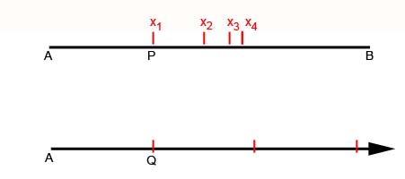
Napier's definition of logarithm is rather interesting. We shall not pursue all its details, but just enough to see its approach and character. Imagine two points, P and L, each moving along its own line.
Figure 3
Figure 3
The line P0 Q is of fixed, finite length, but L's line is endless. L travels along its line at constant speed, but P is slowing down. P and L start (from P0 and L0) with the same speed, but thereafter P's speed drops proportionally to the distance it has still to go: at the half-way point between P0 and Q, P is travelling at half the speed they both started with; at the three-quarter point, it is travelling with a quarter of the speed; and so on. So P is never actually going to get to Q, any more than L will arrive at the end of its line, and at any instant the positions of P and L uniquely correspond. Then at any instant the distance L0L is, in Napier's definition, the logarithm of the distance PQ. (That is, the numbers measuring those distances.) Thus the distance L has travelled at any instant is the logarithm of the distance P has yet to go.
How does this cohere with the ideas we spoke of earlier? The point L moves in an arithmetic progression: there is a constant difference between the distance it moves in equal time intervals – that is what ‘constant speed’ means. The point P, however, is slowing down in a geometric progression: its motion was defined so that it was the ratio of successive distances that remained constant in equal time intervals.
elfatih
From 2000 to 2010, the US GDP changed from 9.9 trillion to 14.4 trillion
Ok, sure, those numbers show change happened. But we probably want insight into the cause: What average annual growth rate would account for this change?
Immediately, my brain thinks “logarithms” because we’re working backwards from the growth to the rate that caused it. I start with a thought like this:
\displaystyle{\text{logarithm of change} \rightarrow \text{cause of growth} }
A good start, but let’s sharpen it up.
First, which logarithm should we use?
By default, I pick the natural logarithm. Most events end up being in terms of the grower (not observer), and I like “riding along” with the growing element to visualize what’s happening. (Radians are similar: they measure angles in terms of the mover.)
Next question: what change do we apply the logarithm to?
We’re really just interested in the ratio between start and finish: 9.9 trillion to 14.4 trillion in 10 years. This is the same growth rate as going from $9.90 to $14.40 in the same period.
We can sharpen our thought:
\displaystyle{\text{natural logarithm of growth ratio} \rightarrow \text{cause of growth} }
\displaystyle{\ln(\frac{14.4}{9.9}) = .374}
Ok, the cause was a rate of .374 or 37.4%. Are we done?
Not yet. Logarithms don’t know about how long a change took (we didn’t plug in 10 years, right?). They give us a rate as if all the change happened in a single time period.
The change could indeed be a single year of 37.4% continuous growth, or 2 years of 18.7% growth, or some other combination.
From the scenario, we know the change took 10 years, so the rate must have been:
\displaystyle{ \text{rate} = \frac{.374}{10} = .0374 = 3.74\%}
From the viewpoint of instant, continuous growth, the US economy grew by 3.74% per year.
Are we done now? Not quite!
This continuous rate is from the grower’s perspective, as if we’re “riding along” with the economy as it changes. A banker probably cares about the human-friendly, year-over-year difference. We can figure this out by letting the continuous growth run for a year:
\displaystyle{\text{exponent with rate and time} \rightarrow \text{effect of growth} }
\displaystyle{e^{\text{rate} \cdot \text{time}} = \text{growth}}
\displaystyle{e^{.0374 \cdot 1} = 1.0381}
The year-over-year gain is 3.8%, slightly higher than the 3.74% instantaneous rate due to compounding. Here’s another way to put it:
From an instant-by-instant basis, a given part of the economy is growing by 3.74%, modeled by e.0374 · years
On a year-by-year basis, with compounding effects worked out, the economy grows by 3.81%, modeled by 1.0381years
In finance, we may want the year-over-year change which can be compared nicely with other trends. In science and engineering, we prefer modeling behavior on an instantaneous basis.
Scenario: Describing Natural Growth
I detest contrived examples like “Assume bacteria doubles every 24 hours, find its growth formula.”. Do bacteria colonies replicate on clean human intervals, and do we wait around for an exact doubling?
A better scenario: “Hey, I found some bacteria, waited an hour, and the lump grew from 2.3 grams to 2.32 grams. I’m going to lunch now. Figure out how much we’ll have when I’m back in 3 hours.”
Let’s model this. We’ll need a logarithm to find the growth rate, and then an exponent to project that growth forward. Like before, let’s keep everything in terms of the natural log to start.
The growth factor is:
\displaystyle{\text{logarithm of change} \rightarrow \text{cause of growth} }
\displaystyle{\ln(\text{growth}) = \ln(2.32/2.3) = .0086 = .86\%}
That’s the rate for one hour, and the general model to project forward will be
\displaystyle{\text{exponent with rate and time} \rightarrow \text{effect of growth} }
\displaystyle{e^{.0086 \cdot \text{hours}} \rightarrow \text{effect of growth} }
If we start with 2.32 and grow for 3 hours we’ll have:
\displaystyle{2.32 \cdot e^{.0086 \cdot 3} = 2.38}
Just for fun, how long until the bacteria doubles? Imagine waiting for 1 to turn to 2:
\displaystyle{1 \cdot e^{.0086 \cdot \text{hours}} = 2}
We can mechanically take the natural log of both sides to “undo the exponent”, but let’s think intuitively.
If 2 is the final result, then ln(2) is the growth input that got us there (some rate × time). We know the rate was .0086, so the time to get to 2 would be:
\displaystyle{ \text{hours} = \frac{\ln(2)}{\text{rate}} = \frac{.693}{.0086} = 80.58}
The colony will double after ~80 hours. (Glad you didn’t stick around?)
What Does The Perspective Change Really Mean?
Figuring out whether you want the input (cause of growth) or output (result of growth) is pretty straightforward. But how do you visualize the grower’s perspective?
Imagine we have little workers who are building the final growth pattern (see the article on exponents):
compound interest
If our growth rate is 100%, we’re telling our initial worker (Mr. Blue) to work steadily and create a 100% copy of himself by the end of the year. If we follow him day-by-day, we see he does finish a 100% copy of himself (Mr. Green) at the end of the year.
But… that worker he was building (Mr. Green) starts working as well. If Mr. Green first appears at the 6-month mark, he has a half-year to work (same annual rate as Mr. Blue) and he builds Mr. Red. Of course, Mr. Red ends up being half done, since Mr. Green only has 6 months.
What if Mr. Green showed up after 4 months? A month? A day? A second? If workers begin growing immediately, we get the instant-by-instant curve defined by ex:
continuous growth
The natural log gives a growth rate in terms of an individual worker’s perspective. We plug that rate into ex to find the final result, with all compounding included.
Using Other Bases
Switching to another type of logarithm (base 10, base 2, etc.) means we’re looking for some pattern in the overall growth, not what the individual worker is doing.
Each logarithm asks a question when seeing a change:
Log base e: What was the instantaneous rate followed by each worker?
Log base 2: How many doublings were required?
Log base 10: How many 10x-ings were required?
Here’s a scenario to analyze:
Over 30 years, the transistor counts on typical chips went from 1000 to 1 billion
How would you analyze this?
Microchips aren’t a single entity that grow smoothly over time. They’re separate editions, from competing companies, and indicate a general tech trend.
Since we’re not “riding along” with an expanding microchip, let’s use a scale made for human convenience. Doubling is easier to think about than 10x-ing.
With these assumptions we get:
\displaystyle{\text{logarithm of change} \rightarrow \text{cause of growth} }
\displaystyle{\log_2(\frac{\text{1 billion}}{1000}) = \log_2(\text{1 million}) \sim \text{20 doublings}}
The “cause of growth” was 20 doublings, which we know occurred over 30 years. This averages 2/3 doublings per year, or 1.5 years per doubling — a nice rule of thumb.
From the grower’s perspective, we’d compute ln(1 billion/1000)/30 years=46% continuous growth (a bit harder to relate to in this scenario).
We can summarize our analysis in a table:
exponents transistor example
Summary
Learning is about finding the hidden captions behind a concept. When is it used? What point view does it bring to the problem?
My current interpretation is that exponents ask about cause vs. effect and grower vs. observer. But we’re never done; part of the fun is seeing how we can recaption old concepts.
Happy math.
Appendix: The Change Of Base Formula
Here’s how to think about switching bases. Assuming a 100% continuous growth rate,
ln(x) is the time to grow to x
ln(2) is the time to grow to 2
Since we have the time to double, we can see how many would “fit” in the total time to grow to x:
\displaystyle{\text{number of doublings from 1 to x} = \frac{\ln(x)}{\ln(2)} = \log_2(x)}
For example, how many doublings occur from 1 to 64?
Well, ln(64) = 4.158. And ln(2) = .693. The number of doublings that fit is:
\displaystyle{\frac{\ln(64)}{\ln(2)} = \frac{4.158}{.693} = 6}
In the real world, calculators may lose precision, so use a direct log base 2 function if possible. And of course, we can have a fractional number: Getting from 1 to the square root of 2 is “half” a doubling, or log2(1.414) = 0.5.
Changing to log base 10 means we’re counting the number of 10x-ings that fit:
\displaystyle{\text{number of 10x-ings from 1 to x} = \frac{\ln(x)}{\ln(10)} = \log_{10}(x) }
dark of the stars
I (a non-mathematician fan of the subject) was suddenly seized with a desire to know how e was implicit in Napier's construction. Your article is the most lucid explanation I could find. Thanks heaps!