Hunting and being hunted

Imagine a forest with humidity hanging in the air. The dense canopy cuts the sunlight out deeming only the leaves and vines hanging from the trees visible. And skulking amongst the shade lays a snake patiently waiting for its prey — a frog. It senses one nearby but still cannot spot it. Why? Is it because the snake has poor eyesight or that the frog has some trick up its sleeve?

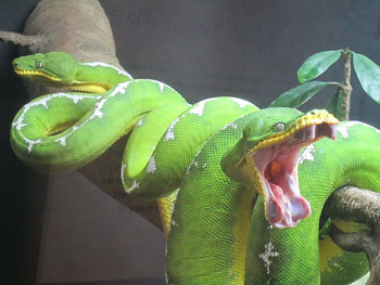
Beware little frog! Tree boas feast on tree frogs. Image: Nate J E,CC BY-SA 3.0.

It turns out that the frog belongs to a species known as the red-eyed frogs. These frogs have neon-green bodies, a unique trait serving as a camouflage by mimicking the color of leaves. In the wake of imminent danger, the frogs flash their red eyes to startle their predators and evade capture. Consequently, the snakes become vulnerable as they are denied food, leading to their population to decline. The frogs survive using their effective camouflage technique and breed, exceeding the snake population over time — producing an ecological imbalance in the rainforest community.

The ecological dynamics of population rise, decline and their fluctuations has attracted the interest of mathematicians for decades. In the 1900s, scientists Alfred J. Lotka and Vito Volterra converted this classical population biology problem into a simple mathematical model.

The classical predator-prey model

The classical predator-prey model was first developed during the World War I. Volterra's motivation was based on an observation made by his colleague during the time of war — that commercial fishing decreased in the Adriatic Sea to a rather low level. Associated with this was an unexpected increase in the population of predators in the sea, that is sharks. Volterra correctly perceived that this was due to fluctuations in the populations of their prey. The idea led up to a model which uses differential equations.

The equations in the original predator-prey model describe how the densities of the prey ( $x$ ) and predator ( $y$ ) populations change over time. The first equation describes the rate of change of the prey population over time

$\frac{dx}{dt} = ax-bxy$

and the rate of change of the predator population is described by

$\frac{dy}{dt} = -cy+dxy.$

The interaction term $xy$ captures the likelihood of an encounter between predator and prey.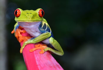

The red-eyed tree frog agalychnis callidryas.

The growth rate of the prey population is represented by the positive coefficient $a$ . To denote the decline of prey population when encountered by predators, the interaction term is multiplied by a negative coefficient $-b$ . On the other hand, the predator flourishes when it interacts with copious amounts of prey, denoted by the positive interaction coefficient $d$ . However, in the absence of prey, predators cannot survive and will decline, a fact captured by the negative coefficient $-c.$

What would eventually happen to this biological system over a long period of time? Would it be able to sustain fluxes in population densities? Can it be envisioned mathematically? We can answer these questions by studying what is known as the steady state or the equilibrium state of the system over time.

The steady state of the prey is determined by evaluating the condition where prey density remains unchanged over time. In other words, the rate of change of prey density is equated to zero, that is $\frac{dx}{dt} = 0.$ Using this condition in equation (1) yields the steady state (mathematically also referred as the fixed point) $y = a/b$ (dashed horizontal line in figure 1a below). How does the prey population dynamically change or flow around the fixed point?

Equation (1) shows that as long as $ax > 0$ (so the existing prey population is not $0$ and prone to grow) and as long as $y < a/b,$ the rate of change $\frac{dx}{dt}$ is greater than $0.$ This means that as long as the predator population $y$ is below the value $a/b$ the prey density continues to grow. Once the predator population increases to above $a/b,$ however, we have $\frac{dx}{dt} < 0,$ so the prey experiences a decline, indicated by green arrows pointing leftwards in figure 1a.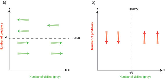

Figure 1

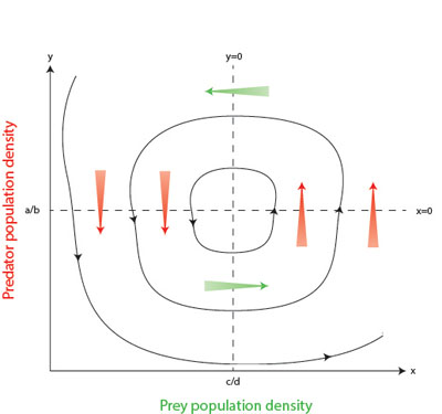
A similar analysis describes the flow for the predator population. The fixed point here is $x = c/d.$ Fig. 1b indicates that the predator population continues to grow (upward arrows) when there is abundance of prey, that is $x>c/d$ (vertical dashed line) and declines (downward arrows) once the prey population decreases below this fixed point, that is $x<c/d.$

Superimposing the flows in prey and predator population gives rise to a typical population cycle indicated in Figure 2.

Figure 2

Modified predator-prey model

One of the assumptions of the previous model is that for each species specific characteristics are homogeneous. For instance, that all frogs share the same skin color. But what happens with additional complexities in the ecological system, in the form of sub-populations of predators and prey, each with distinct features? Examples would be red-eyed frogs versus black-eyed ones or snakes with sharp eyesight versus ones with poor eyesight. Would that not be relevant for their survival?

To understand this, let us consider a situation where some snakes develop sharper eyesight to spot the camouflaged frogs and override the weaker members of their own species. This improved quality of high-offense snakes benefits their survival over their unfit cousins, leading to a decrease in the frog population — even the neon green ones. However, when their food source (frogs) is depleted, this snake sub-population also dwindles. Can the pioneering Lotka-Volterra model be modified to include such a rich repertoire of eco-evolutionary dynamics?

A recent study by a research group led by Michael Cortez at the Georgia Institute of Technology suggests that the answer is yes. The salient feature of the model is that it recapitulates the changes in the community dynamics as a function of co-evolution — wherein both the predator and prey select better survival qualities, dependent on each other.

The modified model

The modified model is based on equations of the form

$\frac{dx}{dt} = F(x,a) - G(x,y,\alpha , \beta )$

$\frac{dy}{dt} = H(x,y,\alpha , \beta ) - D(y,\beta )$

$F,$ $G,$ $H$ and $D$ are mathematical functions chosen to represent growth and death rates and interaction terms. $F$ represents prey growth rate in combination with a function of $\alpha$ chosen to represent the fitness gradients of prey traits. $G$ is the interaction term between predator and prey but is now chosen as a function of the fitness gradients $\alpha$ and $\beta$ of the two species. This term basically determines the prey death rate. $H$ represents the growth rate of the predator in combination with prey interaction and chosen as a function of fitness gradients of both species. $D$ is the predator death rate, in combination with a function of $\beta$ , the fitness gradient of the predator traits.

See the original research paper for more details.

In order to analyse the problem of co-evolution, the scientists created an extended mathematical model, a spin-off of the original version as given in equations (1) and (2) (see the box). The new model includes parameters $\alpha$ and $\beta$ which model the prey and predator sub-populations with their respective survival-reinforcing evolutionary trait values (also called fitness) such as camouflaging attribute of the frogs and sharp eyesight of the snakes. The researchers then used computer simulations to solve the system of equations, resulting in a population cycle shown in figure 3 below.

Let us take the example of frogs and snakes — when there is a population of low vulnerability prey such as the red-eyed frogs (figure 3, red-eyed frogs are represented by shaded green rectangles) interacting with a large population of low offense predators such as snakes with poor eyesight (fig. 3, snakes with bad eyes are represented by open red rectangles) it leads to the event marked 1, with a decline of the predator population. However, this event also drives a selection of increase in high offence snakes with good eyesight (shaded red rectangle), which would then devour the red-eyed frogs (event 2), leading to a decrease in red-eyed frog population (event 3, black-eyed frogs are represented by open green rectangles). Since there are relatively lesser red-eyed frogs now, selection favours low offense predators — snakes with poorer eyesight (event 4) devouring the highly vulnerable frogs (open green rectangle), driving their population down. And the cycle repeats itself.

This cycle is strikingly different from the one resulting from the classical model. A peak in snake population (event 4) is followed by a peak in frog population (event 1). If you didn't know the mechanism behind this pattern, you might think that frogs eat snakes!

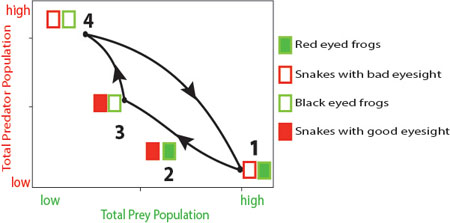
Figure 3

Given this picture, why is it that we do not have all red-eyed frogs and sharp predators — because everything else is unfit for survival? There is something known as a cost associated with maintaining selective survival traits for the species. "An intuitive way to think about costs is to imagine that an organism has a finite amount of energy to spend. For an individual prey, that energy is allocated either towards reproduction (more babies) or more defense (avoiding being eaten by predators). Because high defines prey have a lot of energy invested in defenses, they have less energy invested in reproduction. Thus, the cost for high defense is low reproduction," says Cortez.

How does the new model fit into the broad Darwinian evolutionary paradigm of the survival of the fittest?

"In the cycles, the principle of survival of the fittest is always driving evolution, but because the numbers of prey and predators change over time, the title of 'fittest type' is only held for a short period of time by any given type before it is passed on to a different type. This means that the title of 'fittest type' changes over time," remarks Cortez.

These results show that co-evolution of both predator and prey traits produces novel ecological cycles making this study very relevant to understanding community dynamics. The study defies traditional views that the timescale of evolution is too slow to have an impact on ecological cycles. On the contrary, it reveals that the evolution of survival traits such as frogs with neon green bodies and snakes with sharp eyesight does have an impact in producing short-term changes in the population sizes.

The power of the modified new model lies in intricately capturing subtle changes in fluxes of subpopulations, providing timely and powerful insights into the evolution of organisms. Given the recent Ebola and Zika epidemics, such studies could form the basis of infectious disease models benefiting human healthcare.

About the author

Lakshmi Chandrasekaran has completed her PhD in Mathematical Sciences at the New Jersey Institute of Technology. As an academic researcher, Lakshmi has worked at the interface of mathematics and neuroscience. She freelances as a science writer and editor for an online newspaper The Munich Eye based in Munich, Germany and reports on diverse topics. Currently, she is pursuing a graduate science journalism course at the Medill School of Journalism, Northwestern University, USA.