The maths behind combining R ratios

Although we are now familiar with R, the effective reproduction ratio of a disease, you might also be hearing that R can have different values in different parts of the population. You can think of R as the average number of people an infected person goes on to infect – you can read an introduction to the reproduction ratio here. If you have different values for R for different parts of society – say different geographical regions, or different settings such as hospitals or care homes – you have to consider how these different component parts link together. As you'd expect, this makes the maths more complicated, and we highlighted these difficulties in our previous article. Now, let's look at the maths in more detail.

Let's carry on with the example from that article. In this example, we consider splitting our population into two groups: those who are currently residents, patients or staff in care homes and hospitals, which we'll group under the label "hospital"; and the rest of the population, which we’ll label as the "community". We'll say the reproduction ratio for the community is 0.8, and for hospitals is 0.7. (You can think of these fractional reproduction ratios in this way: a value of 0.8 means that if there are 1000 people with the disease, then on average, they will go on to infect 800 other people.)

We can't consider these two groups in isolation: people from the community move into hospitals when they get sick, and staff from hospitals and care homes can unwittingly take the virus out into the community. We need to consider the transmission of the disease between these two groups. A reasonable assumption is that an infection in the community might go on to cause 0.4 new infections in hospital, and an infection in hospital might go on to cause 0.2 new infections in the community. Now we have four numbers for transmission within, and between hospitals and the community:

Transmission within community $R_{cc} = 0.8$	Transmission from hospital to community $R_{hc}=0.2$
Transmission from community to hospital $R_{ch}=0.4$	Transmission within hospital $R_{hh}=0.7$

If there are 1000 infected people in hospitals and 1000 infected people in the community, then how many new cases of infection will they generate?

A useful heuristic and a warning

Before we dive into the mathematical details, let's look at our example to see what information we can read straight off the table, and when we need to be careful and do the maths in more detail. Adding up the numbers in the left column gives you 1.2, this is the total number of people, on average, an infected person in the community will go on to infect. And adding up the numbers in the right column gives you 0.9, the total number of people an infected person in the hospital will go on to infect, on average. Simply adding up the numbers in the columns in such a table can, in certain circumstances, give you a useful hint of what is going on:

Both columns add up to less than 1: If adding up the numbers in the column comes to less than 1 for both columns – that is any infection will go on to infect less than 1 other person, on average – it's not surprising that we can mathematically show the overall value of R will always be less than 1 and we’d have the disease under control.

Both columns add up to greater than 1: And if the sum of each column was greater than 1, for every column – that is, every infection goes on to infect more than one person, on average – then, again, you wouldn't be surprised to hear that we can show mathematically that the overall value for R will always be greater than 1, and we can be sure new cases of the disease will increase exponentially.

Beware one greater, one less: The tricky situation is when one of the columns adds up to more than 1, and one of the columns to less than 1, just like our example. In this situation you can’t be sure if the disease is under, or out of, control without doing the mathematics required to calculate the overall R.

Down the generations

So we’ve been warned we need to explore our example in a little more mathematical detail. We’ll use the notation $I_ c(0)=1000$ for the original number of infected people in the community, and $I_ h(0)=1000$ for the original number of infected people in hospital. To calculate the 1st generation of new infections in one group, you need the number of new infections produced within that group (ie $R_{cc}I_ c(0)=800$ for new community infections caused by original community infections) and the number of new infections transmitted from the other group (ie $R_{hc}I_ h(0)=200$ for new community infections caused by original infections in hospital). Then the calculations for the 1st generation of new infections in the community, $I_ c(1)$ , and in hospitals, $I_ h(1)$ , are:

$I_ c(1) = R_{cc}I_ c(0) + R_{hc}I_ h(0)=800+200=1000$

$I_ h(1) = R_{ch}I_ c(0) + R_{hh}I_ h(0) = 400+700=1100$

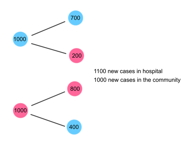
The first generation of new infections for our example.

The 2nd generation of infections can then be calculated from the 1st generation of infections:

$I_ c(2) = R_{cc}I_ c(1) + R_{hc}I_ h(1)=800+220=1020$

$I_ h(2) = R_{ch}I_ c(1) + R_{hh}I_ h(1) = 400+770=1170$

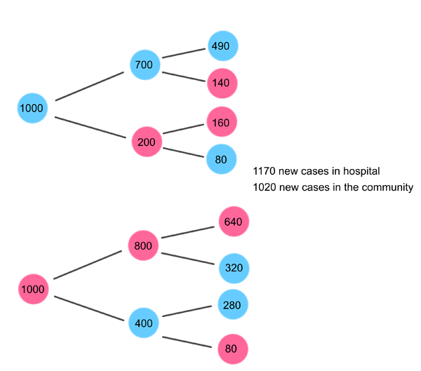
The second round of new infections for our example.

You can carry on this way calculating all future generations of the disease step by step, as we did for the interactivity in the previous article.

But it would be more efficient to skip the intermediate steps, and write the $n$ th generation of infections in terms of the original number of infections. Here’s what that would look like for the 2nd generation of infections:

$\begin{array}{rcl} I_ c(2) & = & R_{cc}I_ c(1) + R_{hc}I_ h(1) \\ & = & R_{cc}(R_{cc}I_ c(0) + R_{hc}I_ h(0)) + R_{hc}(R_{ch}I_ c(0) + R_{hh}I_ h(0)) \\ & = & (R_{cc}^2 +R_{ch}R_{hc})I_ c(0) + (R_{hc}R_{cc} + R_{hh}R_{hc})I_ h(0) \end{array}$

$\text{[math]}$

And

$\begin{array}{rcl} I_ h(2) & = & R_{ch}I_ c(1) + R_{hh}I_ h(1) \\ & = & R_{ch}(R_{hc}I_ h(0) + R_{cc}I_ c(0)) + R_{hh}(R_{hh}I_ h(0) + R_{ch}I_ c(0)) \\ & = & (R_{ch}R_{hh} + R_{cc}R_{ch})I_ c(0) + (R_{hh}^2 +R_{hc}R_{ch})I_ h(0) \end{array}$

$\text{[math]}$

This is only the 2nd generation and it’s already pretty unwieldy. Luckily, if you know a bit of linear algebra from first year university, you might recognise that you can write all these calculations far more simply using matrices and vectors:

$\left( \begin{array}{c} I_ c(1) \\ I_ h(1) \end{array} \right) = \left( \begin{array}{cc} R_{cc} & R_{hc} \\ R_{ch} & R_{hh} \end{array} \right) \left( \begin{array}{c} I_ c(0) \\ I_ h(0) \end{array} \right) = \left( \begin{array}{cc} R_{cc} I_ c(0) + R_{hc} I_ h(0) \\ R_{ch} I_ c(0) + R_{hh} I_ h(0) \end{array} \right)$

and

$\begin{array}{tcl} \left( \begin{array}{c} I_ c(2) \\ I_ h(2) \end{array} \right) & = & \left( \begin{array}{cc} R_{cc} & R_{hc} \\ R_{ch} & R_{hh} \end{array} \right) \left( \begin{array}{c} I_ c(1) \\ I_ h(1) \end{array} \right) \\ & = & \left( \begin{array}{cc} R_{cc} & R_{hc} \\ R_{ch} & R_{hh} \end{array} \right) \left( \begin{array}{cc} R_{cc} & R_{hc} \\ R_{ch} & R_{hh} \end{array} \right) \left( \begin{array}{c} I_ c(0) \\ I_ h(0) \end{array} \right). \\ \end{array}$

This notation gives you a much simpler way to write the calculation for the $n$ th generation of new infections. A simple induction argument shows that:

$\left( \begin{array}{c} I_ c(n) \\ I_ h(n) \end{array} \right) = \left( \begin{array}{cc} R_{cc} & R_{hc} \\ R_{ch} & R_{hh} \end{array} \right) \left( \begin{array}{c} I_ c(n-1) \\ I_ h(n-1) \end{array} \right) = \left( \begin{array}{cc} R_{cc} & R_{hc} \\ R_{ch} & R_{hh} \end{array} \right)^ n \left( \begin{array}{c} I_ c(0) \\ I_ h(0) \end{array} \right),$

which you can write more simply still as

$I(n) = M I(n-1) = M^ n I(0)$

where I(n) is the vector containing the number of new infections in the community, and in hospital, in the nth generation of infection, and M is the next generation matrix consisting of all the transmission rates within and between the groups.

What is the overall R?

Using linear algebra gives you a clearer and more elegant way to describe the growth of the epidemic. It also means you can access the results from this area of maths to explore what happens.

For example, we can find what's called the eigenvalues of the next generation matrix $M$ : these are two numbers, $\lambda _1$ and $\lambda _2$ , with corresponding eigenvectors $v_1$ and $v_2$ , such that multiplying the eigenvector by the matrix is the same as scaling the vector by the eigenvalue:

$Mv_ i = \lambda _ i v_ i$

And you can show by induction, repeatedly applying $M$ to an eigenvector gives you:

$M^ k v_ i = \lambda _ i^ k v_ i.$

Another useful linear algebra fact is that for almost every matrix, the eigenvectors are linearly independent, which means that one eigenvector isn't a linear combination of the others. And, in fact, we can write any arbitrary vector as a linear combination of these two eigenvectors. (You need to allow complex numbers in your eigenvalues and eigenvectors for this fact to be true – you can read more here – but we'll make it clear a little later why we aren't bothered by this.)

That means, you can write our infection vector $I(0)$ , consisting of the original number of infections in the community and hospital, as:

$I(0) = av_1 + bv_2$

Then the next generation of new infections will be:

$I(1) = MI(0)=aMv_1 + bMv_2 = a\lambda _1v_1+b\lambda _2v_2$

And the $n$ th generation of new infections will be:

$I(n)=M^ nI(t)=a\lambda _1^ nv_1+b\lambda _2^ nv_2.$

Another result from linear algebra says that, because the entries in the next generation matrix are all positive real numbers (you can't infect a negative number of people), the "largest" eigenvalue (in terms of its magnitude) will also be a positive real number. We are all now familiar with exponential growth, so you can see how expression for I(n) will quickly be dominated by the term involving that dominant eigenvalue, as the number of generations grows.

In fact, you can show that this dominant eigenvalue is equivalent to the overall value for R for a compartmentalised system represented by such a next generation matrix. And eventually, the system will settle down to a split of infections between the two settings that is represented by the corresponding eigenvector. So for our example, the eigenvalues of the next generation matrix

$\left( \begin{array}{cc} 0.8 & 0.2 \\ 0.4 & 0.7 \end{array} \right)$

are 1.04 and 0.46 (rounded to two decimal places). So the overall R for this compartmentalised population is R=1.04. And after a number of generations of infections, about 45% of the new infections will occur in the community and 55% of the new infections will occur in hospitals, in any future generation of infections. (This is because the dominant eigenvector is (0.84, 1) and 0.84 is 45%, and 1 is 55%, of 1.84, giving the relative proportions of infections across the two groups.)

What we know about R

Our example splits the population into two groups: hospitals (including care homes) and the community. But what if you wanted to differentiate between more groups, say between care homes, hospitals and the community? Or between a number of geographic regions? The mathematics can be extended to a population that is split into any number of groups. The dimension of the next generation matrix (2x2 in our model) increases to the number of groups, and includes entries for the transmission of infections between any two of the groups, as well as the individual R values for infections generated within each group. And the mathematics we introduced above still works, the overall R for the whole population is the dominant eigenvalue for the next generation matrix.

As we intuitively explored in our previous article, the value of the overall R for any compartmentalised population is always greater than the value of any of the individual numbers in the next generation matrix. This can be proved mathematically for a population split into any number of groups. Calculating the dominant eigenvalue, the overall R, is straightforward using linear algebra but isn't easy to do in your head. The important thing to remember, as we demonstrated with our example in the illustration above, is even if the values for transmission between and within the groups are all less than 1, the overall R may still be greater than one. You have to do the maths to be sure.

About this article

Rachel Thomas and Marianne Freiberger are the Editors of Plus, and they produced this article in collaboration with Julia Gog, Professor of Mathematical Biology at the University of Cambridge.